Next: Genetic Fuzzy Systems
Up: GBML Areas
Previous: Evolving Neural Networks
Contents
Subsections
3.5 Learning Classifier Systems
3.5 Learning Classifier Systems
Learning Classifier Systems (LCS) originated in the GA community as a
way of applying GAs to learning problems. The LCS field is one of the
oldest, largest and most active areas of GBML.
The majority of LCS research is currently carried out on XCS
[301,50] and its derivatives XCSF
[305,306] for regression/function approximation
and UCS [23,222] for supervised
learning.
Terminology has been contentious in
this area [121]. LCS are also widely simply called
Classifier Systems (abbreviated CS or CFS) and sometimes evolutionary
(learning) classifier systems. At one time GBML referred exclusively
to LCS. None of these names is very satisfactory but the field appears
to have settled on LCS.
The difficulty in naming the field relates in part to the difficulty
in defining what an LCS is [254,126]. In
practise, what is accepted as an LCS has become more inclusive over
the years. A reasonable definition of an LCS would be an evolutionary
rule-based system - except that a significant minority of LCS are not
evolutionary! On the other hand, most non-evolutionary rule-based
systems are not considered LCS, so the boundaries of the field are
defined more by convention than principle. Even EA practitioners are
far from unanimous; work continues to be published which some would
definitely consider forms of LCS, but which make no reference to the
term and which contain few or no LCS references.
(L)CS has at times been taken to refer to Michigan systems only (see
e.g. [111]) but it now generally includes Pitt systems
as well, as implied by the name and content of IWLCS - the
International Workshop on Learning Classifier Systems - which
includes both Pitt and Michigan, evolutionary and non-evolutionary
systems.
As a final terminological note, rules in LCS are often referred to as
``classifiers''.
3.5.1 Production Systems and Rule(Set) Parameters
LCS evolve condition-action (IF-THEN) rules. Recall from
§2.2 and figure 2 that
in Michigan rule-based systems a chromosome is a single rule while in
Pittsburgh systems a chromosome is a variable-length set of
rules.
Pittsburgh, Michigan, IRL and GCCL are all used. Michigan systems are
rare elsewhere but are the most common form of LCS. Within LCS, IRL is
most common with fuzzy systems, but see [4] for a
non-fuzzy version.
In LCS, we typically evolve rule conditions and actions although
non-evolutionary operators may act upon them. In addition, each
phenotype has parameters associated with it and these parameters are
typically learned rather than evolved using the Widrow-Hoff update or
similar (see [178] for examples).
In Michigan LCS parameters are associated with each rule but in
Pittsburgh systems they are associated with each ruleset. For example,
in UCS the parameters are: fitness, mean action set size (to bias a
deletion process which seeks to balance action set sizes) and
experience (a count of the number of times a rule has been applied, in
order to estimate confidence in its fitness). In GAssist (a supervised
Pittsburgh system) the only parameter is fitness.
Variations of the above exist; in some cases rules predict the next
input or read and write to memory.
3.5.2 Representation
The most common representation in LCS uses fixed-length strings with
binary inputs and outputs and ternary condition. In a simple Michigan
version (see e.g. [301]) each rule has one action and
one condition from  where # is a wildcard, matching both
0 and 1 in inputs. For example, the condition 01# matches two inputs:
010 and 011. Similar representations were used almost exclusively
prior to approximately 2000 and are inherited from GAs and their
preference for minimal alphabets. (Indeed, ternary conditions have an
interesting parallel with ternary schemata [235] for
binary GAs.) Such rules individually have limited expressive power
[248] (but see also [28]) which
necessitates that solutions are sets of rules. More insidiously, the
lack of individual expressiveness can be a factor in pathological
credit assignment (strong/fit overgenerals
[154]). Various extensions to the simple scheme described
above have been studied (see [154] §2.2.2).
where # is a wildcard, matching both
0 and 1 in inputs. For example, the condition 01# matches two inputs:
010 and 011. Similar representations were used almost exclusively
prior to approximately 2000 and are inherited from GAs and their
preference for minimal alphabets. (Indeed, ternary conditions have an
interesting parallel with ternary schemata [235] for
binary GAs.) Such rules individually have limited expressive power
[248] (but see also [28]) which
necessitates that solutions are sets of rules. More insidiously, the
lack of individual expressiveness can be a factor in pathological
credit assignment (strong/fit overgenerals
[154]). Various extensions to the simple scheme described
above have been studied (see [154] §2.2.2).
Following [13]
(p. 87) we distinguish two approaches to real-valued interval
representation in conditions. The first is representations based on
discretisation: HIDER* uses natural coding [107],
ECL clusters attribute values and evolves constraints on them
[82] while GAssist uses adaptive discretisation
intervals [13]. The second approach is to handle
real values directly. In HIDER (unlike HIDER*) genes specify a lower and upper bound
(where lower is always less than upper) [4]. In
[73] a variation of HIDER's scheme is used where the
attribute is ignored when the upper bound is less than the
lower. Interval representations are also used in
[298,264]. Finally [303] specifies
bounds using centre and spread genes.
Various forms of
default/exception rule structures have been used with LCS. It has been
argued that they should increase the number of solutions possible
without increasing the search space and should allow gradual
refinement of knowledge by adding exceptions
[127]. However, the the space of combinations of
rules is much larger than the set of rules and the evolutionary
dynamics of default/exception rule combinations has proved difficult
to manage in Michigan systems. Nonetheless, default rules can
significantly reduce the number of rules needed for a solution
[282] and there have been some
successes. Figure 8 illustrates three
representations for a Boolean function. The leftmost is a truth table,
which lists all possible inputs and their outputs. The middle
representation is the ternary language commonly used by LCS, which
requires only four rules to represent the eight input/output pairs,
thanks to the generalisation provided by the # symbol. Finally, on
the right a default rule (###  1) has been added to the
ternary representation. This rule matches all inputs and states that
the output is always 1. This rule is incorrect by itself, but the two
rules above it provide exceptions and, taken together, the three
accurately represent the function using one less rule than the middle
representation. One difficulty in evolving such default/exception
structures lies in identifying which rules are the defaults and which
the exceptions; a simple solution is to maintain the population in
some order and make earlier rules exceptions to later ones (as in a
decision list [237]). This is straightforward in Pitt
systems in which individual rulesets are static but is more complex in
Michigan populations in which individual rules are created and deleted
dynamically. The other issue is how to assign credit to the overall
multi-rule structure. In Pittsburgh systems this is again
straightforward since fitness is assigned only at the level of
rulesets, but in Michigan systems each rule has a fitness, and it is
not obvious how to credit the three rules in the default/exception
structure in a way which recognises their cooperation.
1) has been added to the
ternary representation. This rule matches all inputs and states that
the output is always 1. This rule is incorrect by itself, but the two
rules above it provide exceptions and, taken together, the three
accurately represent the function using one less rule than the middle
representation. One difficulty in evolving such default/exception
structures lies in identifying which rules are the defaults and which
the exceptions; a simple solution is to maintain the population in
some order and make earlier rules exceptions to later ones (as in a
decision list [237]). This is straightforward in Pitt
systems in which individual rulesets are static but is more complex in
Michigan populations in which individual rules are created and deleted
dynamically. The other issue is how to assign credit to the overall
multi-rule structure. In Pittsburgh systems this is again
straightforward since fitness is assigned only at the level of
rulesets, but in Michigan systems each rule has a fitness, and it is
not obvious how to credit the three rules in the default/exception
structure in a way which recognises their cooperation.
Figure 8:
Three representations for the 3 multiplexer function
![\begin{figure}\begin{center}
\begin{tabular}{\vert ccc\vert c\vert} \hline
\mu...
...\rightarrow$}\condWorker 1] \ \hline
\end{tabular}
\end{center}\end{figure}](img15.png) |
The Pittsburgh GABIL [144] and GAssist
[13] use decision lists and often evolve default rules
spontaneously (e.g. a fully general last rule). Bacardit found that
enforcing a fully general last rule in each ruleset in GAssist (and
allowing evolution to select the most useful class for such rules) was
effective [13].
In Michigan systems default/exception structures are called default
hierarchies. Rule specificity has been used as the criterion for
determining which rules are exceptions and accordingly conflict
resolution methods have been biased according to specificity. There
are, however, many problems with this approach [258]. It is
difficult for evolution to produce these structure since they depend
on cooperation between otherwise competing rules. The structures are
unstable since they are interdependent; unfortunate deletion of one
member alters the utility of the entire structure. As noted they
complicate credit assignment and conflict resolution since exception
rules must override defaults [299,258].
There are also problems with the use of specificity to prioritise
rules. For one, having fewer #s does not mean a rule actually
matches fewer inputs; counting #s is a purely syntactic measure of
generality. For another, there is no reason why exception rules should
be more specific.
The consequence of these difficulties is that there has not been much
interest in Michigan default hierarchies since the early 1990s (but
see [285]) and indeed not all Michigan LCS support them
(e.g. ZCS [300], XCS/XCSF and UCS do not). Nonetheless,
the idea should perhaps be revisited and an ensembles perspective
might prove useful.
A great
range of other representations have been used, particularly in recent
years. These include VL logic [206] as used in GIL
[140], first-order logic
[203,204,205], decision lists as used in
GABIL [144] and GAssist [13], messy
encoding [172], ellipses [51] and
hyperellipses [57], hyperspheres [200],
convex hulls [187], tile coding [177] and a
closely related hyperplane coding [30,29], GP
trees [5,173,174], Boolean networks
defined by GP [38], support vectors [198],
edges of an Augmented Transition Network [170], Gene
Expression Programming [309], fuzzy rules (see
§3.6) and neural networks
[257,75,259,41,211,76,131,130].
GALE [194,193,197] has used particularly
complex representations, including the use of GP to evolve trees
defining axis-parallel and oblique hyper-rectangles [197],
and evolved prototypes which are used with a k-nearest-neighbour
classifier. The prototypes need not be fully specified; some
attributes can be left undefined. This representation has also been
used in GAssist [13].
There has been limited work with alternative action representations
including computed actions [278,186] and continuous
actions [308].
logic [206] as used in GIL
[140], first-order logic
[203,204,205], decision lists as used in
GABIL [144] and GAssist [13], messy
encoding [172], ellipses [51] and
hyperellipses [57], hyperspheres [200],
convex hulls [187], tile coding [177] and a
closely related hyperplane coding [30,29], GP
trees [5,173,174], Boolean networks
defined by GP [38], support vectors [198],
edges of an Augmented Transition Network [170], Gene
Expression Programming [309], fuzzy rules (see
§3.6) and neural networks
[257,75,259,41,211,76,131,130].
GALE [194,193,197] has used particularly
complex representations, including the use of GP to evolve trees
defining axis-parallel and oblique hyper-rectangles [197],
and evolved prototypes which are used with a k-nearest-neighbour
classifier. The prototypes need not be fully specified; some
attributes can be left undefined. This representation has also been
used in GAssist [13].
There has been limited work with alternative action representations
including computed actions [278,186] and continuous
actions [308].
Evolutionary Selection of Representations
As we have seen there are many representations to chose
from. Unfortunately it is generally not clear which might be best for
a given problem or part of a problem. One approach is to let evolution
make these choices. This can be seen as a form of meta-learning in
which evolution adapts the inductive bias of the learner.
In [13,14] evolution was used to select
default actions in decision lists in GAssist. GAssist's initial
population was seeded with last rules which together advocated all
possible classes and over time evolution selected the most suitable of
these rules. To obtain good results it was necessary to encourage
diversity in default actions.
In GALE [193] evolution selects both classification
algorithms and representations. GALE has elements Cellular Automata
and Artificial Life: individuals are distributed on a 2-dimensional
grid. Only neighbours within  cells interact: two neighbours may
perform crossover, an individual may be cloned and copied to a
neighbouring cell, and an individual may die if its neighbours are
fitter. A number of representations have been used: rule sets,
prototypes, and decision trees (orthogonal, oblique, and multivariate
based on nearest neighbor). Decision trees are evolved using GP while
prototypes are used by a k-nearest-neighbour algorithm to select
outputs. An individual uses a particular representation and
classification algorithm and hence evolutionary selection operates on
both. Populations may be homogeneous or heterogeneous and in
[197] GALE was modified to interbreed orthogonal and
oblique trees.
cells interact: two neighbours may
perform crossover, an individual may be cloned and copied to a
neighbouring cell, and an individual may die if its neighbours are
fitter. A number of representations have been used: rule sets,
prototypes, and decision trees (orthogonal, oblique, and multivariate
based on nearest neighbor). Decision trees are evolved using GP while
prototypes are used by a k-nearest-neighbour algorithm to select
outputs. An individual uses a particular representation and
classification algorithm and hence evolutionary selection operates on
both. Populations may be homogeneous or heterogeneous and in
[197] GALE was modified to interbreed orthogonal and
oblique trees.
In the representational ecology approach [200]
condition shapes were selected by evolution. Two Boolean
classification tasks were used: a plane function which is easy to
describe with hyperplanes but hard with hyperspheres, and a sphere
function which has the opposite characteristics.
Three versions of XCS were used: with hyperplane conditions
(XCS-planes), with hyperspheres (XCS-spheres), and both (XCS-both).
XCS was otherwise unchanged, but in XCS-both the representations
compete due to XCS's pressure against overlapping
rules [154].
In XCS-both planes and spheres do not interbreed; they constitute
genetically independent populations, that is, species. In terms of
classification accuracy XCS-planes did well on the plane function and
poorly on the sphere function while XCS-sphere showed the opposite
results. XCS-both performed well on both; there was no significant
difference in accuracy compared to the better single-representation
version on each problem. Furthermore, XCS-both selected the more
appropriate representation for each function. In terms of the amount
of training needed, XCS-both was similar to XCS-sphere on the sphere
function but was significantly slower than XCS-plane on the plane
function.
GAssist's
Adaptive Discretization Intervals (ADI) approach has two parts
[13]. The first consists of adapting interval
sizes. To begin, a discretisation algorithm proposes cut points for
each attribute and this defines the finest discretisation possible,
said to be composed of micro-intervals. Evolution can merge and split
macro-intervals, which are composed of micro-intervals, and each
individual can have different macro-intervals. The second part
consists of selecting discretisation algorithms. Evolution is allowed
to select discretisation algorithms for each attribute or rule from a
pool including uniform-width, uniform-frequency, ID3, Fayyad and
Irani, Màntaras, USD, ChiMerge and random. Unfortunately, evolving
the best discretisers was found to be difficult and the use of ADI
resulted in only small improvements in accuracy. However, further work
was suggested.
In [301] Wilson introduced an optimisation for Michigan
populations called macroclassifiers. He noted that as an XCS
population converges on the solution set many identical copies of this
set accumulate. A macroclassifier is simply a rule with an additional
numerosity parameter which indicates how many identical virtual
rules it represents. Using macroclassifiers saves a great deal of
run-time compared to processing a large number of identical rules.
Furthermore, macroclassifiers provide interesting statistics on
evolutionary dynamics. Empirically macroclassifiers perform
essentially as the equivalent `micro'classifiers [151].
Figure 9 illustrates how the rules m and m in the top can be represented by m alone in the bottom by adding a
numerosity parameter.
in the top can be represented by m alone in the bottom by adding a
numerosity parameter.
Figure 9:
A population of microclassifiers (top) and the equivalent macroclassifiers (bottom)
![\begin{figure}\begin{center}
\begin{tabular}{c c c c} \hline
{\bf Rule} & {\bf...
... 001110] & \condWorker 1] & 100.0 & 1
\end{tabular} \end{center}
\end{figure}](img19.png) |
3.5.3 Rule Discovery
LCS are interesting from an evolutionary perspective, particularly
Michigan systems in which evolutionary dynamics are more complex than
in Pittsburgh systems. Where Pittsburgh systems face two objectives
(evolving accurate and parsimonious rulesets) Michigan systems face a
third: coverage of the input (or input/output) space. Furthermore,
Michigan systems have coevolutionary dynamics as rules both cooperate
and compete. Since the level of selection (rules) is lower than the
level of solutions (rulesets) researchers have attempted to coax
better results by modifying rule fitness calculations with various
methods. Fitness sharing and crowding have been used to encourage
diversity and hence coverage. Fitness sharing is naturally based on
inputs (see ZCS) while crowding has been implemented by making
deletion probability proportional to the degree of overlap with other
rules (as in XCS). Finally, restricted mating as implemented by a
niche GA plays an important role in XCS and UCS (see §3.5.3).
Windowing in Pittsburgh LCS
As noted in §2.2
naive implementations of the Pittsburgh approach are slower than
Michigan systems, which are themselves slow compared to
non-evolutionary methods. The naive Pitt approach is to evaluate each
individual on the entire data set but much can be done to improve
this. Instead, windowing methods [99] learn on
subsets of the data to improve runtime. Windowing has been used in
Pitt LCS since at least ADAM [113]. More recently GAssist
used ILAS (Incremental Learning by Alternating Strata)
[13] which partitions the data into  strata, each
with the same class distribution as the entire set. A different
stratum is used for fitness evaluation each generation. On larger data
sets speed-up can be an order of magnitude. Windowing has become a
standard part of recent Pittsburgh systems applied to real-world
problems (e.g. [15,11,10]).
strata, each
with the same class distribution as the entire set. A different
stratum is used for fitness evaluation each generation. On larger data
sets speed-up can be an order of magnitude. Windowing has become a
standard part of recent Pittsburgh systems applied to real-world
problems (e.g. [15,11,10]).
Many ensemble methods improve classification accuracy by sampling data
in similar ways to windowing techniques which suggests the potential
for both improved accuracy and run-time but this has not been
investigated in LCS.
Most rule discovery work focuses
on Michigan LCS as they are more common and their evolutionary
dynamics are more complex. The rest of this section deals with
Michigan systems although many ideas, such as self-adaptive mutation,
could be applied to Pitt systems. Michigan LCS use the steady-state
GAs introduced in §2.4 as they minimise disruption to the
rule population during on-line learning.
An unusual feature of Michigan LCS is the emphasis placed on
minimising population size, for which various techniques are use:
niche GAs, the addition of a generalisation term in fitness,
subsumption deletion, condensation and various compaction methods.
Niche GAs
Whereas in a standard panmictic GA all rules are
eligible for reproduction, in a niche GA mating is restricted to rules
in the same action set (which is considered a niche). (See figure
3 on action sets.) The inputs spaces of
rules in an action set overlap and their actions agree, which suggests
their predictions will tend to be related. Consequently, mating these
related rules is more effective, on average, than mating rules drawn
from the entire population. This is a form of speciation since it
creates non-interbreeding sub-populations.
However, the niche GA has many other effects
[301]. First, a strong bias towards general rules, since
they match more inputs and hence appear in more action sets. Second,
pressure against overlapping rules, since they compete for
reproduction [154]. Third, complete coverage of the input
space, since competition occurs for each input.
The niche GA was introduced in [27] and originally
operated in the match set but was later further restricted to the
action set [302]. It is used in in XCS and UCS and is
related to universal suffrage [106].
Recently Butz et
al. [59,58,60] replaced XCS's usual
crossover with an an Estimation of Distribution Algorithm (EDA)-based method to
improve solving of difficult hierarchical problems while
[195,196] introduced CCS: a Pitt LCS based on
compact GAs (a simple form of EDA).
A rule  logically subsumes a rule
 when matches a superset of the inputs matches and they
have the same action. For example, 00#0 subsumes 000
0 and 001 0. In XCS is allowed to
subsume if: i) logically subsumes , ii) is sufficiently
accurate and iii) is sufficiently experienced (has been evaluated
sufficiently) so we can have confidence in its accuracy.
Subsumption deletion was introduced in XCS (see [50]) and
takes two forms. In GA subsumption, when a child is created we
check to see if its parents subsume it, which constrains accurate
parents to only produce more general children. In action set
subsumption, the most general of the sufficiently accurate and
experienced rules in the action set is given the opportunity to
subsume the others. This removes redundant, specific rules from the
population but is too aggressive for some problems.
when matches a superset of the inputs matches and they
have the same action. For example, 00#0 subsumes 000
0 and 001 0. In XCS is allowed to
subsume if: i) logically subsumes , ii) is sufficiently
accurate and iii) is sufficiently experienced (has been evaluated
sufficiently) so we can have confidence in its accuracy.
Subsumption deletion was introduced in XCS (see [50]) and
takes two forms. In GA subsumption, when a child is created we
check to see if its parents subsume it, which constrains accurate
parents to only produce more general children. In action set
subsumption, the most general of the sufficiently accurate and
experienced rules in the action set is given the opportunity to
subsume the others. This removes redundant, specific rules from the
population but is too aggressive for some problems.
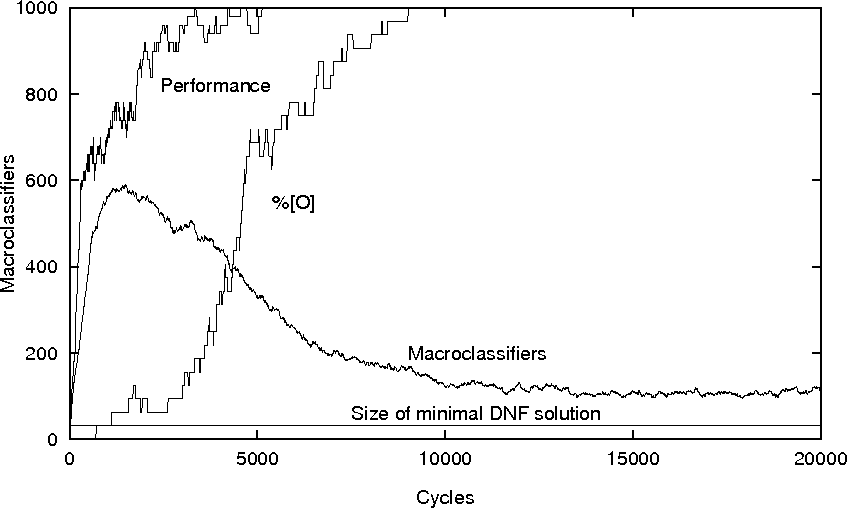
Michigan LCS have
interesting evolutionary dynamics and plotting macroclassifiers is a
useful way to monitor population convergence and parsimony. Figure
10 illustrates by showing XCS learning the 11
multiplexer function. The performance curve is a moving average of the
proportion of the last 50 inputs which were classified correctly,
%[O] shows the proportion of the minimal set of 16 ternary rules XCS
needs to represent this function (indicated by the straight line
labelled ``Size of minimal DNF solution'' in the figure) and
macroclassifiers were explained in §3.5.2.
In this experiment the population was initially empty and was seeded
by covering §3.5.3. ``Cycles'' refers to the number of
inputs presented, inputs were drawn uniform randomly from the input
space, the population size limit was 800, all input/output pairs were
in both the train and test sets, GA subsumption was used but action
set subsumption was not and curves are the average of 10 runs. Other
settings are as in [301].
Figure 10:
Evolutionary dynamics of XCS on the 11 multiplexer
|
|
Note that XCS continues to refine its solution (population) after
100% performance is reached and that it finds the minimal
representation (at the point where %[O] reaches the top of the
figure) but that continued crossover and mutation generate extra
transient rules which make the population much larger.
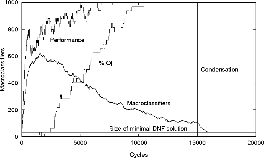
As illustrated by figure
10 an evolved population normally contains many
redundant and low-fitness rules. These rules are typically transient,
but more are generated while the GA continues to run. Condensation
[301,151] is a very simple technique to remove such rules
which consists of running the system with crossover and mutation
turned off; we only clone and delete existing rules. Figure
11 repeats the experiment from figure
10 but switches after 15,000 cycles to condensation
after which the population quickly converges to the minimal solution.
Other methods of compacting the population have been investigated
[152,307,84].
Figure 11:
XCS with condensation on the 11 multiplexer
|
|
XCS is robust to class
imbalances [217] but for very high imbalances
tuning the GA based on a facetwise model improved performance
[217,219].
Self-tuning evolutionary search has also been studied. The mutation
rate can be adapted during evolution
e.g. [133,134,131,61], while
[79] dynamically controls use of two generalisation
operators: each has a control bit specifying whether it can be used
and control bits evolve with the rest of the genotype.
Evolution has been
supplemented by heuristics in various ways. Covering, first suggested
in [124], creates a rule to match an unmatched input.
It can be used to an create (``seed'') the initial population
[287,301,122] or to supplement the
GA throughout evolution [301]. Kovacs [154]
(p. 42) found covering each action set was preferable to covering the
match set when applying XCS to sequential tasks. Most covering/seeding
is done as needed but instead [190] selects inputs at the
center of same-class clusters.
For other non-evolutionary operators see
[27,236], the work on corporations of rules
[310,255,276,275,277],
and the work on non-evolutionary LCS.
Although LCS were originally
conceived as a way of applying GAs to learning problems
[128], not all LCS include a GA. Various heuristics have
been used to create and refine rules in e.g. YACS [103]
and MACS [102].
A number of systems have been inspired by psychological models of
learning. ACS [263,47] and ACS2 [46]
are examples, although ACS was also later supplemented by a GA
[48,49]. Another is AgentP, a specialised LCS for
maze tasks [321,320].
While credit assignment in Pittsburgh LCS is a straightforward matter
of multi-objective fitness evaluation, as noted in §3.5.3 it is far more complex in Michigan
systems with their more complex evolutionary dynamics. Credit
assignment is also more complex in some learning paradigms,
particularly reinforcement learning, which we will not cover
here. Within supervised learning credit assignment is more complex in
regression tasks than in classification. These difficulties have been
the major issue for Michigan LCS and have occupied a considerable part
of the literature, particularly prior to the development of XCS which
provided a reasonable solution for both supervised and reinforcement
learning.
Although we are not
covering reinforcement learning work, Michigan LCS have traditionally
been designed for such problems. XCS/XCSF are reinforcement learning
systems but since supervised learning can be formulated as simplified
reinforcement learning they have been applied to SL
tasks. Consequently, we now very briefly outline the difference
between the two major forms of Michigan reinforcement learning LCS.
In older (pre-1995) reinforcement learning LCS fitness is proportional
to the magnitude of reward and is called strength. Strength is
used both for conflict resolution and as fitness in the GA (see
e.g. ZCS [300]). Such LCS are referred to as
strength-based and they suffer from many difficulties with credit
assignment [154], the analysis of which is quite complex.
Although some strength-based systems incorporate accuracy as a
component of fitness, their fitness is still proportional to reward.
In contrast, the main feature of XCS is that it adds a prediction
parameter which estimates the reward to be obtained if the action
advocated by a rule is taken. Rule fitness is proportional to the
accuracy of reward prediction and not to its magnitude which avoids
many problems strength-based systems have with credit assignment. In
XCS accuracy is estimated from the variance in reward and since
overgeneral rules have high variance they have low fitness. Although
XCS has proved robust in a range of applications, a major limitation
is that the accuracy estimate conflates several things: i)
overgenerality in rules, ii) noise in the training data and iii)
stochasticity in the transition function in sequential problems. In
contrast, strength-based systems may be less affected by noise and
stochasticity since they are little affected by reward variance. See
[154] for analysis of the two approaches.
To update rule predictions while
training, the basic XCS system [301,50] uses the
Widrow-Hoff update for non-sequential problems and the Q-learning
update for sequential ones. Various alternatives have been used:
average rewards [271,185], gradient descent
[55,184] and eligibility traces
[89].
The basic XCSF uses NLMS (linear piecewise) prediction
[305,306] but Lanzi [178] has
compared various alternative classical parameter estimation (RLS and
Kalman filter) and gain adaptation algorithms (K1, K2, IDBD, and IDD).
He found that Kalman filter and RLS have significantly better accuracy
than the others and that Kalman filter produces more compact solutions
than RLS.
There has also been recent work on other systems; UCS is essentially a
supervised version of XCS and the main difference is its prediction
update. Bull has also studied simplified LCS [40].
In
[179] Lanzi selects prediction functions in XCSFHP (XCSF
with Heterogeneous Predictors) in a way similar to the selection of
condition types in the representational ecology approach in
§3.5.2. Polynomial functions (linear,
quadratic and cubic) and constant, linear and NN predictors were
available. XCSFHP selected the most suitable predictor for regression
and sequential tasks and performed almost as well as XCSF using the
best single predictor.
Theoretical Results
Among the
notable theoretical works on LCS, [175] demonstrates that
XCS without generalisation implements tabular Q-learning,
[54] investigates the computational complexity of XCS in a
Probably Approximately Correct (PAC) setting, and
[291,290,289,292] analyse credit
assignment and relate LCS to mainstream reinforcement learning
methods. [154] identifies pathological rule types: strong
overgeneral and fit overgeneral rules which are overgeneral yet
stronger/fitter than not-overgeneral competitors. Fortunately such
rules are only possible under specific circumstances.
A number of papers seek to characterise problems which are hard for
LCS
[110,156,153,154,24,16]
while others model evolutionary dynamics
[45,53,52,56,220,221]
and others attempt to reconstruct LCS from first principles using
probabilistic models
[91,90,92].
Hierarchical LCS have
been studied for some time and [18] reviews early
work. [88] and
[86,87,85] apply hierarchical LCS
to robot control while [19] uses hierarchical XCSs to
learn long sequences of actions.
The ensembles field §3.3 studies how to
combine predictions [167] and all the above could be
reformulated as ensembles of LCS. There has been some recent work on
ensembles of LCS [77,39] and also treating a single
LCS as an ensemble [36,90,92].
LCS face certain inherent difficulties; Michigan
systems face complex credit assignment problems while in Pittsburgh
systems run-time can be a major issue. The same is true for all GBML
systems, but the Michigan approach has been explored far more
extensively within LCS than elsewhere. Recently there has been much
integration with mainstream machine learning and much research on
representations and credit assignment algorithms. Most recent
applications have been to data mining and function approximation
although some work continues on reinforcement learning. Future
directions are likely to include exposing more of the LCS to evolution
and further integration with machine learning, ensembles, memetic
algorithms and multi-objective optimisation.
No general up-to-date introduction to LCS
exists. For the basics see [109] and the introductory
parts of [154] or [52]. For a good
introduction to representations and operators see chapter 6 of
[95]. For a review of early LCS see
[19]. For reviews of LCS research see
[310,180,176]. For a review of
state-of-the-art GBML and empirical comparison to non-evolutionary
pattern recognition methods see [224]. For other
comparisons with non-evolutionary methods see
[26,114,244,304,22,23].
Finally, the LCS bibliography [155] has over 900 references.
Next: Genetic Fuzzy Systems
Up: GBML Areas
Previous: Evolving Neural Networks
Contents
T Kovacs
2011-03-12