Next: Learning Classifier Systems
Up: GBML Areas
Previous: Evolving Ensembles
Contents
Subsections
3.4 Evolving Neural Networks
3.4 Evolving Neural Networks
The study of Neural Networks (NNs) is a large and interdisciplinary
area. The term Artificial Neural Network (ANN) is often used to
distinguish simulations from biological NNs, but having noted this we
shall refer simply to NNs. When evolution is involved such systems may
be called EANNs (Evolving Artificial Neural Networks) [316]
or ECoSs (Evolving Connectionist Systems) [147].
A neural network consists of a set of nodes, a set of directed
connections between a subset of nodes and a set of weights on the
connections. The connections specify inputs and outputs to and from
nodes and there are three forms of nodes: input nodes (for input to
the network from the outside world), output nodes, and hidden nodes
which only connect to other nodes. Nodes are typically arranged in
layers: the input layer, hidden layer(s) and output layer.
Nodes compute by integrating their inputs using an activation function
and passing on their activation as output. Connection weights modulate
the activation they pass on and in the simplest form of learning
weights are modified while all else remains fixed. The most common
approach to learning weights is to use a gradient descent-based
learning rule such as backpropagation.
The architecture of a NN refers to the set of nodes,
connections, activation functions and the plasticity of nodes; whether
they can be updated or not. Most often all nodes use the same
activation function and in virtually all cases all nodes can be
updated.
Evolution has been applied at three levels: weights, architecture and
learning rules. In terms of architecture, evolution has been used to
determine connectivity, select activation functions, and determine
plasticity.
Three forms of representation have been
used: i) direct encoding [316,93] in which all
details (connections and nodes) are specified, ii) indirect encoding
[316,93] in which general features are specified
(e.g. number of hidden layers and nodes) and a learning process
determines the details, and iii) developmental encoding
[93] in which a developmental process is genetically
encoded
[149,115,210,135,225,268].
Implicit and developmental representations are more flexible and tend
to be used for evolving architectures while direct representations
tend to be used for evolving weights alone.
Evolving NNs virtually always use the
Pittsburgh approach although there are a few Michigan systems:
[6,256,259]. In Michigan systems each
chromosome specifies only one hidden node which raises issues. How
should the architecture be defined? A simple method is to fix it in
advance. How can we make nodes specialise? Two options are to
encourage diversity during evolution, e.g. with fitness sharing, or
after evolution, by pruning redundant nodes [6].
Most NN learning rules are based on
gradient descent, including the best known: backpropagation (BP). BP
has many successful applications, but gradient descent-based methods
require a continuous and differentiable error function and often get
trapped in local minima [267,294].
An alternative is to evolve the weights which has the advantages that
EAs don't rely on gradients and can work on discrete fitness
functions.
Another advantage of evolving weights is that the same evolutionary
method can be used for different types of network (feedforward,
recurrent, higher order), which is a great convenience for the
engineer [316]. Consequently, much research has been done
on evolution of weights.
Unsurprisingly fitness functions penalise NN error but they also
typically penalise network complexity (number of hidden nodes) in
order to control overfitting. The expressive power of a NN depends on
the number of hidden nodes: fewer nodes = less expressive = fits
training data less while more nodes = more expressive = fits data
better. As a result, if a NN has too few nodes it underfits while with
too many nodes it overfits.
In terms of training rate there is no clear winner between evolution
and gradient descent; which is better depends on the problem
[316]. However, Yao [316] states that evolving
weights AND architecture is better than evolving weights alone and
that evolution seems better for reinforcement learning and recurrent
networks. Floreano [93] suggests evolution is better
for dynamic networks. Happily we don't have to choose between the two
approaches.
Evolution is good at finding
a good basin of attraction but poor at finding the optimum of the
basin. In contrast, gradient descent has the opposite
characteristics. To get the best of both [316] we should
evolve initial weights and then train them with gradient
descent. [93] claims this can be two orders of
magnitude faster than beginning with random initial weights.
Architecture has an important
impact on performance and can determine whether a NN under- or
over-fits. Designing architectures by hand is a tedious, expert,
trial-and-error process. Alternatives include constructive NNs which
grow from a minimal network and destructive NNs which shrink from a
maximal network. Unfortunately both can become stuck in local optima
and can only generate certain architectures [7].
Another alternative is to evolve architectures. Miller et
al. [207] make the following suggestions (quoted from
[316]) as to why EAs should be suitable for searching the
space of architectures.
- The surface is infinitely large since the number of possible
nodes and connections is unbounded;
- the surface is nondifferentiable since changes in the number of
nodes or connections are discrete and can have a discontinuous
effect on EANN's performance;
- the surface is complex and noisy since the mapping from an
architecture to its performance is indirect, strongly epistatic, and
dependent on the evaluation method used;
- the surface is deceptive since similar architectures may have
quite different performance;
- the surface is multimodal since different architectures may
have similar performance.
There are good reasons to evolve architectures and weights
simultaneously. If we learn with gradient descent there is a
many-to-one mapping from NN genotypes to phenotypes [318].
Random initial weights and stochastic learning lead to different
outcomes, which makes fitness evaluation noisy, and necessitates
averaging over multiple runs, which means the process is slow.
On the other hand, if we evolve architectures and weights
simultaneously we have a one-to-one genotype to phenotype mapping
which avoids the problem above and results in faster learning.
Furthermore, we can co-optimise other parameters of the network
[93] at the same time. For example, [21]
found the best networks had a very high learning rate which may have
been optimal due to many factors such as initial weights, training
order, and amount of training. Without co-optimising architecture and
weights evolution would not have been able to take all factors into
account at the same time.
There is no one
best learning rule for all architectures or problems. Selecting rules
by hand is difficult and if we evolve the architecture then we don't a
priori know what it will be. A way to deal with this is to evolve the
learning rule, but we must be careful: the architectures and problems
used in learning the rules must be representative of those to which it
will eventually be applied. To get general rules we should train on
general problems and architectures, not just one kind. On the other
hand, to obtain a training rule specialised for a specific
architecture or problem type, we should train just on that
architecture or problem.
One approach is to evolve only learning rule parameters
[316] such as the learning rate and momentum in
backpropagation. This has the effect of adapting a standard learning
rule to the architecture or problem at hand. Non-evolutionary methods
of adapting training rules also exist. Castillo [66],
working with multi-layer perceptrons, found evolving the architecture,
initial weights and rule parameters together as good or better than
evolving only first two or the third.
We can also evolve new learning rules
[316,233]. Open-ended evolution of rules was initially
considered impractical and instead Chalmers [67]
specified a generic, abstract form of update and evolved its
parameters to produce different concrete rules. The generic update was
a linear function of ten terms, each of which had an associated
evolved real-valued weight. Four of the terms represented local
information for the node being updated while the other six terms were
the pairwise products of the first four. Using this method Chalmers
was able to rediscover the delta rule and some of its variants. This
approach has been used by a number of others and has been reported to
outperform human-designed rules [78].
More recently, GP was used to evolve novel types of rules from a set
of mathematical functions and the best new rules consistently
outperformed standard backpropagation [233].
Whereas architectures are fixed, rules could potentially change over
their lifetime (e.g. their learning rate could change) but evolving
dynamic rules would naturally be much more complex than evolving
static ones.
Most methods output a single NN [317]
but a population of evolving NNs is naturally treated as an ensemble
and recent work has begun to do so. Evolving NNs is inherently
multiobjective: we want accurate yet simple and diverse networks. Some
work combines these objectives into one fitness function while others
is explicitly multi-objective.
Yao [319] used
EPNet's [318] population as an ensemble without modifying the
evolutionary process. By treating the population as an ensemble the
result outperformed the population's best individual.
Liu and Yao [191] pursued accuracy and diversity in two
ways. The first was to modify backpropagation to minimise error and
maximise diversity using an approach they call Negative Correlation
Learning (NCL) in which the errors of members become negatively
correlated and hence diverse. The second method was to combine
accuracy and diversity in a single objective.
EENCL (Evolutionary Ensembles for NCL) [192] automatically
determines the size of an ensemble. It encourages diversity with
fitness sharing and NCL and it deals with the ensemble member
selection problem §3.3.1 with a
cluster-and-select method (see [142]). First we cluster
candidates based on their errors on the training set so that clusters
of candidates make similar errors. Then we select the most accurate
in each cluster to join the ensemble; the result is the ensemble can
be much small than the population.
CNNE (Cooperative Neural Net Ensembles) [138] used a
constructive approach to determine the number of individuals and how
many hidden nodes each has. Both contribute to the expressive power of
the ensemble and CNNE was able to balance the two to obtain suitable
ensembles. Unsurprisingly it was found that more complex problems
needed larger ensembles.
MPANN (Memetic Pareto Artificial
NN) [2] was the first ensemble of NNs to use
multi-objective evolution. It also uses gradient-based local search to
optimise network complexity and error.
DIVACE (diverse and accurate ensembles) [68] uses
multiobjective evolution to maximise accuracy and diversity.
Evolutionary selection is based on non-dominated sorting
[261], a cluster-and-select approach is used to form
the ensemble, and search is provided by simulated annealing and a
variant of differential evolution [265].
DIVACE-II [69] is a heterogeneous multiobjective
Michigan approach using NNs, Support Vector Machines and Radial Basis
Function Nets. The role of crossover and mutation is played by bagging
[33] and boosting [97] which produce
accurate and diverse candidates. Each generation bagging and boosting
makes candidate ensemble members and only dominated members are
replaced. The accuracy of DIVACE-II was very good compared to 25 other
learners on the Australian credit card and diabetes datasets and it
outperformed the original DIVACE.
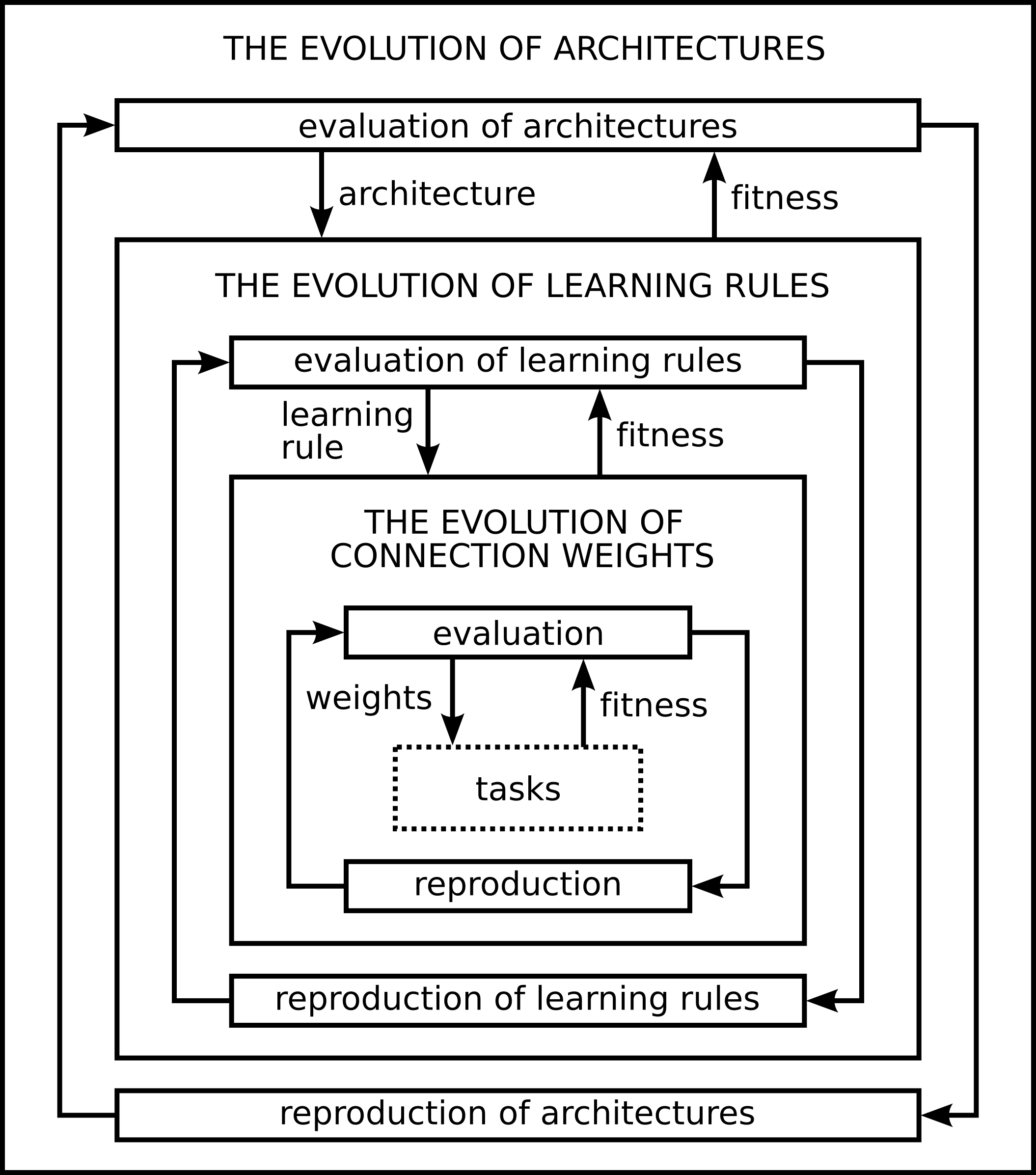
Figure 7 shows Yao's
framework for evolving architectures, training rules and weights as
nested processes [316]. Weight evolution is innermost as it
occurs at the fastest time scale while either rule or architecture
evolution is outermost. If we have prior knowledge, or are interested
in a specific class of either rule or architecture, this constrains
the search space and Yao suggests the outermost should be the one
which constrains it most. The framework can be thought of as a
3-dimensional space of evolutionary NNs where 0 on each axis
represents one-shot search and infinity represents exhaustive
search. If we remove references to EAs and NNs it becomes a general
framework for adaptive systems.
Figure 7:
Yao's framework for evolving architectures, training rules and weights
|
|
Evolution is widely used with NNs, indeed according to Floreano et al.
[93] most studies of neural robots in real environments
use some form of evolution. Floreano et al. go on to claim evolving
NNs can be used to study ``brain development and dynamics because it
can encompass multiple temporal and spatial scales along which an
organism evolves, such as genetic, developmental, learning, and
behavioral phenomena. The possibility to co-evolve both the neural
system and the morphological properties of agents ...adds an
additional valuable perspective to the evolutionary approach that
cannot be matched by any other approach.'' [93] (p. 59).
Key reading on evolving NNs includes Yao's classic
1999 survey [316], Kasabov's 2007 book, Floreano, Dürr
and Mattiussi's 2008 survey [93] which includes reviews
of evolving dynamic and neuromodulatory NNs, and Yao and Islam's 2008
survey of evolving NN ensembles [317].
Next: Learning Classifier Systems
Up: GBML Areas
Previous: Evolving Ensembles
Contents
T Kovacs
2011-03-12