2.2 Classifying GBML Systems Algorithmically

In the Pittsburgh (Pitt) approach one chromosome encodes one solution. We assume fitness is assigned to chromosomes, so in Pitt systems it is assigned to solutions. This leaves a credit assignment problem: how did the chromosome's component genes contribute to the observed fitness of the chromosome? This is left to evolution as this is what EAs are designed to deal with. In the Michigan approach one solution is (typically) represented by many chromosomes and so fitness is assigned to partial solutions. Credit assignment differs from the Pitt case as chromosomes not only compete for reproduction but may also complement and cooperate with each other. This gives rise to the issues of how to encourage cooperation, complementarity, and coverage of inputs, all of which makes designing an effective fitness function more complex than in Pitt systems. In Michigan systems the credit assignment problem is how to measure a chromosome's contributions to the overall solution, as reflected in the various aspects of fitness just mentioned. To sum up the difficulty in Michigan systems: the best set of chromosomes may not be the set of best (i.e. fittest) chromosomes [95]. 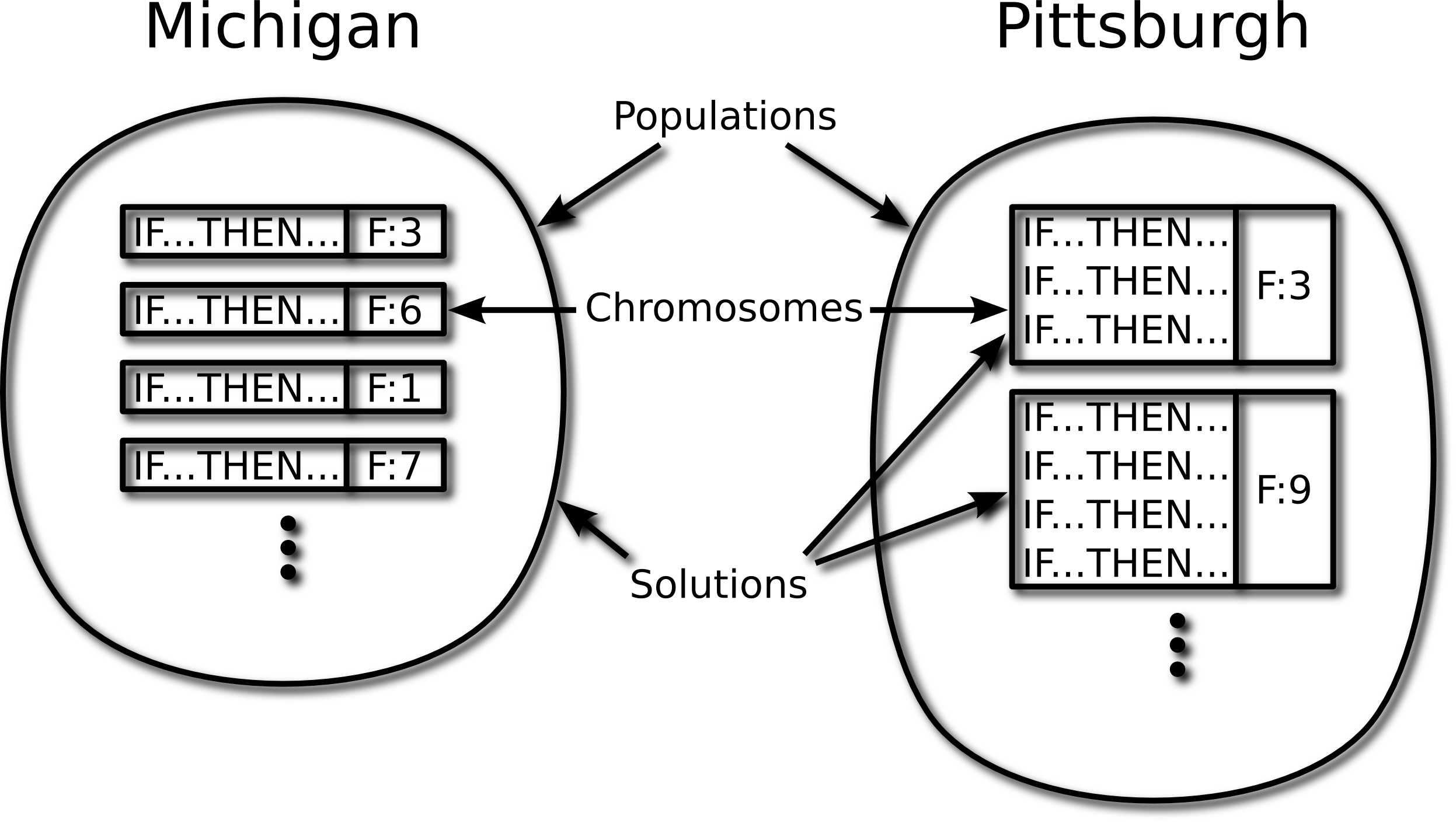To illustrate, figure 2 depicts the representation used by Pitt and Michigan versions of the rule-based systems called Learning Classifier Systems (see §3.5). In a Pittsburgh LCS a chromosome is a variable-length set of rules while in a Michigan LCS a chromosome is a single fixed-length rule.

Figure 2: Michigan and Pittsburgh rule-based systems compared. The F:$x$ associated with each chromosome indicates its fitness

Although the Pittsburgh and Michigan approaches are generally presented as two discrete cases some hybrids exist e.g. [297].

Pittsburgh and Michigan Compared

Pittsburgh systems (especially naive implementations) are slower, since they evolve more complex structures and they assign credit at a less specific (and hence less informative) level.¹Additionally, since their chromosomes are more complex so are their genetic operators. On the other hand they face less complex credit assignment problems and are hence more robust, that is, more likely to adapt successfully. Michigan systems use a finer grain of credit assignment than the Pittsburgh approach, which means bad partial solutions can be deleted without restarting from scratch. This makes them more efficient and also more suitable for incremental learning. However, credit assignment is more complex in Michigan systems. Since the solution is a set of chromosomes: i) the population must not converge fully, and ii) as noted the best set of chromosomes may not be the set of best chromosomes.

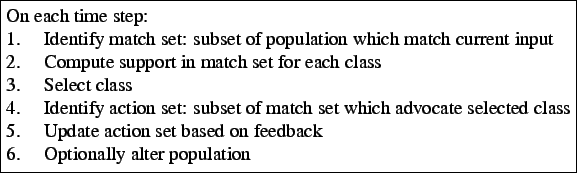
The two approaches also tend to be applied in different ways. Pitt systems are typically used offline and are algorithm-driven; the main loop processes each chromosome in turn and seeks out data to evaluate them (which is how a standard GA works, although fitness evaluation is typically simpler in a GA). In contrast, Michigan systems are typically used online and are data-driven; the main loop processes each data input in turn and seeks out applicable chromosomes (see figure 3). As a result Michigan systems are more often used as learners (though not necessarily more often as meta-learners) for reinforcement learning, which is almost always on-line. The Michigan approach has mainly been used with LCS. See [111,141,297,96,154] for comparison of the approaches.

Figure 3: A basic Michigan algorithm

Iterative Rule Learning

IRL is a variation on the Michigan approach in which, as usual, one solution is represented by many chromosomes, but only the single best chromosome is selected after each run, which alters the co-evolutionary dynamics of the system. The output of multiple runs is combined to produce the solution. The approach originated with SIA (Supervised Inductive Algorithm) [287,190], a supervised genetic rule learner.

Genetic Cooperative-Competitive Learning

GCCL is another Michigan approach in which on each generation is ranked by fitness and a coverage-based filter then allocates inputs to the first rule which correctly covers them. Inputs are only allocated to one rule per generation and rules which have no inputs allocated die at the end of a generation. The remaining rules' collective accuracy is compared to the previous best generation, which is stored offline. If the new generation is more accurate (or the same but has fewer rules) it replaces the previous best. Examples include COGIN [111,112], REGAL [105], and LOGENPRO [312].