|
|
Topology-Preserving Selection and Clustering (TPSC)
GO TO ➢ [ Summary · Vector Space Model · SOM · SVD ] ➢ [ Hybrid SOM-SVD · Two-Phase Clustering ] ➢ [ HOWTO ] ➢ [ Citations ]
SOM
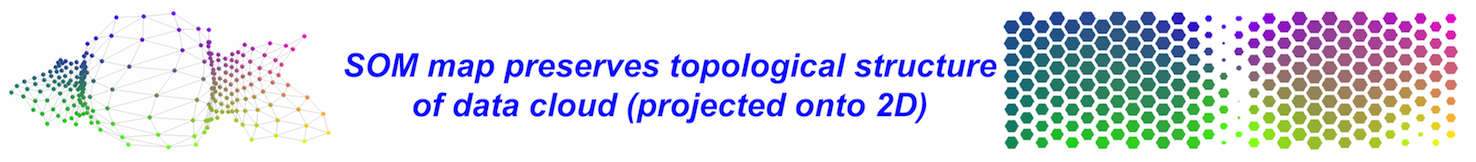
To capture such topological structure of the expression data, self-organizing map (SOM) can be competent in preserving local and global topological properties (Tamayo et al., 1999; Kohonen, 2001; Xiao et al., 2003). This unsupervised non-linear algorithm configures output vectors into a topological preservation of the input high-dimensional data in a non-linear manner, producing a SOM map in which genes with the same or similar expression patterns can be mapped to the same or nearby map nodes. The topology of this SOM map follows and reflects the topological structure of input data. More importantly, the SOM algorithm quantizes the training input data (vector quantization, VQ) and carries out a non-linear topological preserving projection (vector projection, VP) in an interactive manner, allowing smoother neighborhood kernels to define the extent of regularization that VP exerts on the VQ (Kohonen, 2001). In addition to the visual benefits provided by the ordered map (Xiao et al., 2003; Fang et al., 2008), the output matrix of SOM with an appropriate neighborhood kernel may be more powerful than the expression matrix for exploratory analyses. Depending on the specific questions being addressed, neighborhood kernels can be geared to tasks such as the topology-preserving pre-processing and characterization of microarray data.
Topology of SOM Artificial neuronal network-based SOM mimics the data structure of the input space by converting the nonlinear relationships between input vectors into simple geometric relationships on a regular two-dimensional hexagonal grid of map nodes. Each node is represented by two kinds of vectors: the location vector on the two-dimensional map grid, and the prototype vector in the high-dimensional hyperspace. Typically, the topology of SOM is heuristically determined based on the input training data. Given a gene expression matrix (G × N) as input, the number M of nodes (i.e., the product of the side lengths of the map grid) is initially calculated based on the heuristic formula M=5 x sqrt(G). Then, the ratio between the side lengths is set to the square root of the two biggest eigenvalues of the training data. Therefore, the actual side lengths are then finely set so that their product is as close to M as possible.
|
|