3.2 Genetic Programming

Genetic Programming (GP) is a major evolutionary paradigm which evolves programs [286]. The differences between GP and GAs are not precise but typically GP evolves variable-length structures, typically trees, in which genes can be functions. See [314] for discussion. [95] discusses differences between GAs and GP which arise because GP representations are more complex. Among the pros of GP: i) it is easier to represent complex languages, such first-order logic, in GP, ii) it is easier to represent complex concepts compactly, and iii) GP is good at finding novel, complex patterns overlooked by other methods. Among the cons of GP: i) expressive representations have large search spaces, ii) GP tends to overfit / does not generalise well, and iii) variable-length representations suffer from bloat (see e.g. [231]).

While GAs are typically applied to function optimisation, GP is widely applied to learning. To illustrate, of the set of ``typical GP problems'' defined by Koza [158], which have become more-or-less agreed benchmarks for the GP community [286], there are many learning problems. These include the multiplexer and parity Boolean functions, symbolic regression of mathematical functions and the Intertwined Spirals problem, which involves classification of 2-dimensional points as belonging to one of two spirals. GP usually follows the Pittsburgh approach. We cover the two representations most widely used for learning with GP: GP trees and decision trees.

3.2.1 GP Trees

GP Trees for Classification

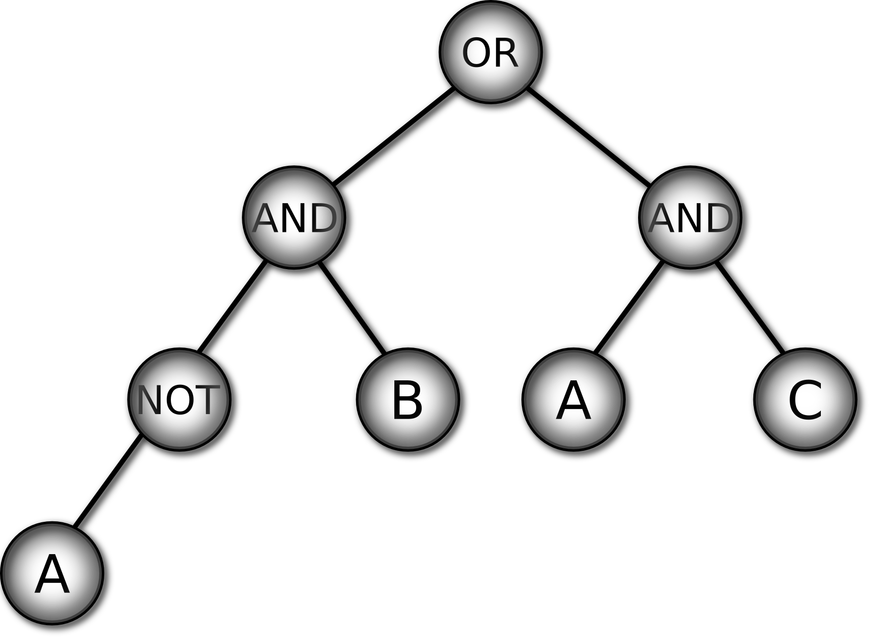
Figure 4 shows the 3 multiplexer Boolean function as a truth table on the left and as a GP tree on the right. To classify an input with the GP tree: i) instantiate the leaf variables with the input values, ii) propagate values upwards from leaves though the functions in the non-leaf nodes and iii) output the value of the root (top) node as the classification.

Figure 4: Two representations of the 3 multiplexer function: truth table (left) and GP tree (right)

A	B	C	Class
0	0	0	0
0	0	1	0
0	1	0	1
0	1	1	1
1	0	0	0
1	0	1	1
1	1	0	0
1	1	1	1

GP Trees for Regression

In regression problems leaves may be constants or variables and non-leaves are mathematical functions. Figure 5 shows a real-valued function as an algebraic expression on the left and as a GP tree on the right. (Note that

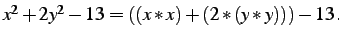$x^2+2y^2-13 = ((x*x)+(2*(y*y)))-13.$) The output of the tree is computed in the same way as in the preceding classification example.

Figure 5: Two representations of a real-valued function

$x^2+2y^2-13$

3.2.2 Decision Trees

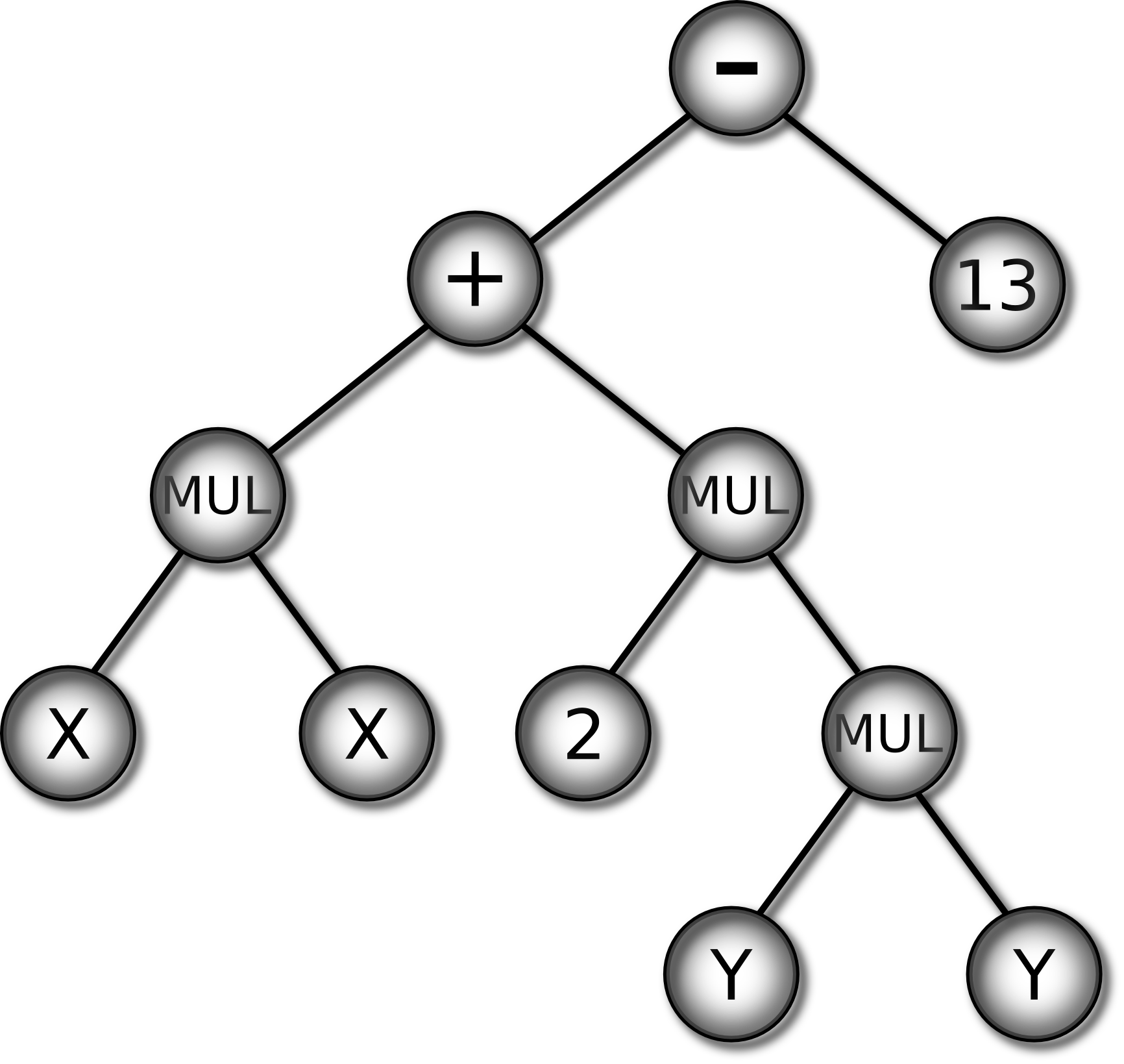Figure 6 shows the 3 multiplexer as a truth table and as a decision tree. To classify an input in such a tree: i) start at the root (top) of tree, ii) follow the branch corresponding to the value of the attribute in the input, iii) repeat until a leaf is reached, and iv) output the value of the leaf as the classification of the input.

Figure 6: Two representations of the 3 multiplexer function: truth table (left) and decision tree (right)

A	B	C	Class
0	0	0	0
0	0	1	0
0	1	0	1
0	1	1	1
1	0	0	0
1	0	1	1
1	1	0	0
1	1	1	1

Evolving First-order Trees

First-order trees use both propositional and first-order internal nodes. [239] found first-order logic made trees more expressive and allowed much smaller solutions than found by the rule learner CN2 or the tree learner C4.5, with similar accuracy.

Oblique (Linear) Trees

Whereas conventional tree algorithms learn axis-parallel decision boundaries, oblique trees make tests on a linear combination of attributes. The resulting trees and more expressive but have a larger search space. See [32].

Evolving Individual Nodes in Decision Trees

In most GP-based tree evolvers an individual is a complete tree but in [199] each individual is a tree node. The tree is built incrementally: one GP run is made for each node. This is similar to IRL in §2.2 but results are added to a tree structure rather than a list.

3.2.3 Extensions to GP

Ensemble Methods and GP

Ensemble ideas have been used in two ways. First, to reduce fitness computation time and memory requirements by training on subsamples of the data. The bagging approach has been used in [94,136] and the boosting approach in [260]. Although not an ensemble technique, the Limited Error Fitness method introduced in [101] as a way of reducing GP run-time works in a similar manner: in LEF the proportion of the training set used to evaluate fitness depends on the individual's performance. The second ensemble approach has improved accuracy by building an ensemble of GP trees. In [148,227] each run adds one tree to the ensemble and weights are computed with standard boosting.

GP Hyperheuristics

Schmidhuber [247] proposed a meta-GP system evolving evolutionary operators as a way of expanding the power of GP's evolutionary search. Instead of evolving decision rules Krasnogor proposes applying GP to the much harder task of evolving classification algorithms, represented using grammars [160,162,163]. Freitas [95] §12.2.3 sketches a similar approach which he calls algorithm induction while in [226] Pappa and Freitas go into the subject at length. [42] also deals with GP hyperheuristics.

3.2.4 Conclusions

Lack of Test Sets in GP

GP terminology follows a convention in the GA field since at least [125] in which brittleness refers to overfitting or poor generalisation to unseen cases, and robustness refers to good generalisation. A feature of the GP literature is that GP is usually evaluated only on the training set [168,286]. Kushchu has also criticised the way in which test sets have been used [168]. Nonetheless GP has the same need for test sets to evaluate generalisation as other methods [168] and as a result the ability of GP to perform inductive generalisation is one of the open issues for GP identified in [286]. See [168,286] for methods which have been used to encourage generalisation in GP, many of which can be applied to other methods.

Reading

See Koza's 1994 book [159] for the basics of evolving decision trees with GP, Wong and Leung's 2000 book on data mining with grammar-based GP [312], Freitas' 2002 book [95] for a good introduction to GP, decision trees and both evolutionary and non-evolutionary learning, Poli, Langdon and McPhee's free 2008 GP book [231], and Vanneschi and Poli's 2010 survey of GP [286]. The GP bibliography has over 5000 entries [171].