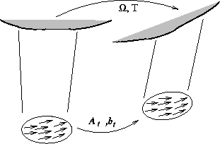
Figure 2: Affine motion tracking
The extraction of the affine estimates has essentially two components: the identification of an appropriate set of 2-D spatial patches to represent each surface in a scene; and the tracking of the patches through the image sequence. The first of these is not considered here; it is assumed that by analysis of the first few frames, patches can be identified corresponding to distinct surfaces. This will necessarily involve using additional information such as colour and scale, as well as motion, and making assumptions about spatial coherency. Although this is by no means a trivial problem, note that it need not be as arduous as a full pixel segmentation of the frames - the number of patches will be relatively small and in the present context of obtaining 3-D motion and structure, they need only provide approximate coverage of the surfaces concerned. This is discussed more fully in [3].
The tracking of the 2-D patches and estimation of their associated affine motion parameters is achieved using weighted linear regression over an estimated optical flow field. The weights are provided by truncated Gaussian windows, each defining the spatial extent of one of the patches being tracked. The choice of a Gaussian window function is deliberate: the group of such functions are closed under the action of affine transformation and hence naturally represent the evolution of the patches as they warp according to the affine motion approximation as illustrated in Fig 2.

Figure 2: Affine motion tracking
For a patch k in frame t, let its affine motion parameters be defined
by the ![]() matrix
matrix ![]() and the
and the ![]() vector
vector
![]() . Given an optical flow estimate
. Given an optical flow estimate ![]() at
position
at
position ![]() , estimates of these parameters are
obtained by using standard least-squares to minimise
, estimates of these parameters are
obtained by using standard least-squares to minimise

where ![]() is the centre of the patch,
is the centre of the patch,
![]() is its Gaussian window defined as
is its Gaussian window defined as
![]()
and ![]() is a local region about
is a local region about ![]() set
according to the extent of the window as defined by the covariance
set
according to the extent of the window as defined by the covariance
![]() . The window centre and covariance evolve according to the
patch's affine motion, hence allowing the patch to be tracked through the
sequence, ie
. The window centre and covariance evolve according to the
patch's affine motion, hence allowing the patch to be tracked through the
sequence, ie
![]()
![]()
where I is the identity and ![]() ,
, ![]() are updated affine motion estimates derived from the EKF as
described in the next section. These provide a link with the 3-D
motion and structure estimation and hence gives a degree of stability
to the tracking. In the experiments the windows were initialised to be
circular in the first frame, ie
are updated affine motion estimates derived from the EKF as
described in the next section. These provide a link with the 3-D
motion and structure estimation and hence gives a degree of stability
to the tracking. In the experiments the windows were initialised to be
circular in the first frame, ie ![]() for some suitable s,
and the optical flow estimates were obtained using the Lucas and
Kanade algorithm [5].
for some suitable s,
and the optical flow estimates were obtained using the Lucas and
Kanade algorithm [5].