|
Julian Gough (Sidney Sussex College)
The bulk of the thesis is concerned with the application of hidden Markov models (HMMs) to remote protein homology detection. The thesis both addresses how best to utilise HMMs, and then uses them to analyse all completely sequenced genomes. There is a structural perspective to the work, and a section on three-dimensional protein structure analysis is included.
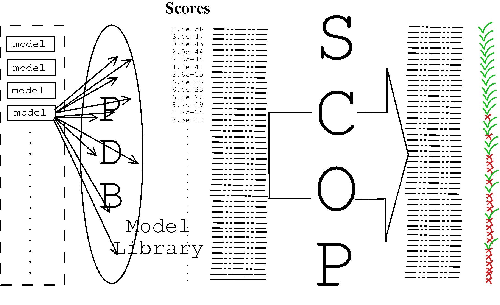
The Structural Classification of Proteins (SCOP) database forms the basis of the structural perspective. SCOP is a hierarchical database of protein domains classified by their structure, sequence and function. The main aim of the work is to use HMMs to classify all protein sequences produced by the genome projects (including human) into their constituent structural domains. To do this HMMs were built to represent all proteins of known structure; the thesis examines ways in which to best do this and describes the construction of a library of models.
Structural domain assignments to the genome sequences were generated by scoring the model library against the genomes, and then selecting the most probable domain architecture for each sequence. The genome assignments (within the framework of the evolutionary-based SCOP classification) provide the capability to study evolution at a molecular level, as well as at the level of the whole organism.
The model library and genome assignments have been made public via the SUPERFAMILY database. The data and services provided have been used for a growing number of projects several of which have already led to publication.
`But I don't want to go among mad people,' Alice remarked.
`Oh, you can't help that,' said the Cat: `we're all mad here. I'm mad. You're mad.'
`How do you know I'm mad?' said Alice.
`You must be,' said the Cat, `or you wouldn't have come here.'
LEWIS CARROL.
When I embarked on this work three years ago I had no previous training in the field. The last biology and chemistry I had done was seven years previously when I was taking my GCSE level exams at the age of sixteen. I thought a protein was something you get when you eat meat, and that an amino acid would probably dissolve plastic or burn your skin. I had never had a computer before and had never heard of Perl or Linux which are the two tools which I have most heavily relied upon for my daily work. So this thesis really describes what a PhD should be, which is a journey of learning; I have also been lucky that my learning has resulted in some interesting science. To preserve the flow of the learning process the work in this thesis is arranged in roughly chronological order.
``Well over 80% of the biological information concerning protein sequences reported in the published literature has been inferred by homology'' [1].
Proteins are the fundamental building blocks of life, and they are completely specified by a simple linear DNA sequence code. Since the invention of dideoxy sequencing [2] it has been very easy to determine these sequences, and millions have already been determined. The rate at which new sequences are being determined is rising faster than that dictated by Moore's law, and more importantly the complete sequences of whole genomes, including the human, are now available.
The sequence alone does not tell us anything about the protein which it codes for. Further information can be obtained by experimentation, but it is very expensive and time consuming. The number of proteins for which there is experimental information is very small relative to the number of proteins for which the sequence is now known. However almost all sequences are homologous to some other sequences, and this homology can be detected using computer algorithms which are very cheap and fast. Therefore information about a large number of sequences can be inferred from knowledge about a small number.
Sequence homology provides reliable information about the large number of sequences being generated by the sequencing projects. The value of this information makes homology methods the most important computational tool in genome biology.
Although sequence analysis easily reveals homology between closely related proteins, structural analysis can be used to detect homology between far more distantly related proteins. Although variation in sequences may have allowed two related proteins to mutate almost all common residues, the three-dimensional core of the protein retains the same main-chain conformation. The conservation of the structure of the core is a requirement for the protein to maintain a stable fold, and hence also a requirement for the protein to remain functional.
It was suggested some time ago that there is a limited repertoire of approximately 1000 protein families [3,4], which has been backed up with stronger evidence more recently [5]. By combining sequence and structure information it should be possible in the future to classify all of the sequences in all of the genomes into this limited number of families. Genome projects have so far supplied us with complete sequence sets, and structural genomics will hopefully soon provide us with structural representatives for every family.
``Nothing in biology makes sense except in the light of evolution'', Theodosius Dobzhansky.
No biological thesis would be complete without mentioning evolution. Having started out with very little biological knowledge I would like to think that I would have independently arrived at the same conclusion as Theodosius Dobzhansky. Although few general conclusions are drawn about evolution in this thesis, the goal of the work from the beginning is to provide necessary information to allow new studies of evolution to be carried out. As a consequence the direction of the thesis is guided by `domains' as minimum evolutionary units, and `superfamilies' as groups of domains sharing a common evolutionary ancestor [6].
The logical progression from this work is to use the results presented here to learn more about the nature of evolution. This is touched upon, but it is really where this thesis ends and future work takes off from [7,8,9].
The first chapter describes the structural analysis of a single protein family. It was important to do this to fully understand the role of structural information in determining the evolutionary relationships of protein domains.
The second chapter is the bulk of the work and investigates the use of hidden Markov model (HMM) technology[10,11,12] for remote protein homology detection. Several key ideas are expressed in this chapter and it sets out the understanding acquired for carrying out the work in the rest of the thesis. It was important to learn about the behaviour of HMMs before they were used to build a model library. Chapter three describes the building of the library of models representing all proteins of known structure [13].
Chapter four takes a sidestep and describes a comparison of different HMM software packages [14,15]. A deeper understanding of HMMs was gained by analysing the performance of the two most commonly used packages.
In chapter five the model library built in chapter three is finally applied; it used to carry out structural domain assignments at the superfamily level to all sequences in the complete genomes. Finally chapter six describes the public server for the model library and genomes assignments.
A simplistic yet systematic approach to sequence homology detection was first developed by Fitch in 1966[16]. This method used a substitution matrix based on the number of nucleotide mutations required to translate between amino acids. This matrix was used to calculate similarity scores for all possible ungapped alignments of a pair of sequences, and hence the significance of the homology. The first systematic sequence comparison procedure which allowed for gaps and insertions in the sequences was published by Needleman and Wunsch in 1970[17]. This work was a major breakthrough at the time, offering the capability to automatically detect homology between much more divergent sequences than was previously possible. Through the use of a dynamic programming algorithm the method was also very efficient, and could be used to compare large numbers of sequences. It was however still very slow compared to the methods subsequently developed. In 1978 major improvements were made to the substitution matrix by Dayhoff and Schwartz[18].
The next major advance was the result of work by Smith and Waterman in 1980[19] which introduced local scoring and included affine gap penalties. An extension to the dynamic programming algorithm developed by Needleman and Wunsch allowed the detection of local similarities, i.e. between subsequences of the pair of whole sequences rather than across the full length of both. This allows for a match between individual domains (subsequences) belonging to larger multi-domain sequences.
The dynamic programming algorithm used by Smith and Waterman guarantees an optimal local alignment, and hence the maximum score, for a given pair of sequences and a substitution matrix. It is however possible to increase the efficiency of the algorithm by adding heuristics which consider a window of residues along the sequence. The optimal alignment is no longer guaranteed but something very close is usually achieved. In 1988 Pearson and Lipman introduced a heuristic method called FASTA[20], and in 1992 another by Altschul and Lipman et al. called BLAST[21]; these offered an increase in efficiency with some loss of sensitivity. Further improvements were made available by Henikoff and Henikoff in 1990, introducing the BLOSSUM substitution matrices[22].
The BLAST and FASTA programs are still in common use, although some continuing work has been done to improve the BLAST algorithm, and the loss in sensitivity due to the heuristics is now far less.
The problem with pair-wise sequence comparison methods is that each position is treated with equal importance and they use the same substitution matrix for every position in the sequence. In reality some positions are far more important than others. For example sites which are in the buried hydrophobic core of a protein are less variable than sites in loop regions on the edge of the protein, and so a difference between a pair of proteins in core residues should be more heavily penalised than at a site on the surface. Furthermore some positions are conserved for different reasons than others, so certain types of substitution should be more heavily penalised than the same type of substitution at a different site.
By considering the 3-dimensional structure of a protein, some of the properties of the residues at each site can be characterised. Information can also be gained by creating a multiple sequence alignment of related sequences, and observing the frequency of the occurance of different residues at each position. These two sources of information can be used together or separately to characterise the features of the sequences at different positions. A position specific scoring matrix (or model) representing these characteristics can be constructed. This is called a profile, and can be used to match and align sequences of far more distantly related proteins than simple pair-wise sequence homology methods.
An early attempt at using a profile to identify protein sequence homology was made by Taylor[23] in 1986. He demonstrates that the use of a profile-based procedure using what he calls ``template fingerprints'' can be used to identify conserved features in immunoglobulin sequences, and attempts to define a general algorithm for the recognition of sequence patterns in globular proteins. The approach used large multiple sequence alignments of variable and constant domains to generate templates representing the conserved features. It was observed that the conserved features were different for immunoglobulins and other beta-sheet proteins. Taylor concludes that ``Matching a new sequence against a data bank of fingerprint templates is potentially a better approach to sequence identification than the current practice of comparing an entire sequence against every other sequence in the databanks ...''. Further template generation and matching was subsequently carried out on the globins by Bashford et al. in 1987[24], but the focus of this work was to identify the sequence features which determine a protein fold, rather than developing a general procedure for sequence alignment and searching. As the conserved features were found to be common to all globins, they were able to distinguish globins from any other sequences.
Growing out of this work in 1987, Gribskov and Eisenberg et al. wrote a program called PROFMAKE[25] and used it to build profiles for globins and immunoglobulins, and search them against a sequence database. This method saw the introduction of position specific gap penalties, and uses a dynamic programming algorithm analogous to that introduced by Needleman and Wunsch for pair-wise sequence comparison. Gribskov and Eisenberg then went on to formally develop programs[26], which Bowie and Eisenberg extended and applied to more families[27].
There still did not exist a robust profile method which could be widely used, until Krogh and Haussler et al. introduced hidden Markov models to computational biology in 1994[10]. Hidden Markov models put the profile methods on firmer mathematical ground by casting the problem within a tight probabilistic framework. This resolved many of the problems associated with profile analysis, improved performance, and by 1996 there were two independent (freely available) software packages being applied to large-scale problems[11]. Without the probabilistic framework provided by the hidden Markov model theory, previous methods had been assigning the position specific scores and gap penalties in a relatively ad hoc manner. The early profile methods could be applied to specific families by tuning the parameters by trial and error, but were unable to achieve the automatic and reliable construction of profiles necessary for them to be applied on a large scale.
The most recent development in the field of profile-based sequence searching which has made a big difference is the use of iterative procedures. In 1997 Altschul and Lipman et al. produced PSI-BLAST[28] which is currently the most commonly used profile-based method. Position Specific Iterated (PSI) BLAST is an improvement, and more importantly, an extension of the original BLAST algorithm. The procedure requires a large database of known protein sequences which it uses to iteratively search for homologues to build a profile from. The initial query sequence is searched against the large database for close homologues, which are then aligned. Position specific score matrices are constructed from the alignment and used to search the database for further homologues not detectable by a pair-wise comparison to the initial query sequence using BLAST. The procedure repeats itself a number of times improving the profile by adding more homologous sequences from the large database to the alignment. The resulting automatically generated profile can be used to search for sequences related to the initial query sequence.
Although the position specific score matrices used by PSI-BLAST are in essence very similar to hidden Markov models, they are somewhat optimised for speed, and lack features such as position specific gap penalties and insertion score matrices. They also fail to make use of the Dirichlet mixtures[29] and null models used by hidden Markov model methods. In 1999 Karplus and Hughey et al. published[14] an iterative hidden Markov model procedure similar to PSI-BLAST, but using hidden Markov models instead of position specific score matrices. There have subsequently been improvements made to PSI-BLAST[30], but a comparison in this thesis, finds the performance of Karplus and Hughey's hidden Markov model procedure SAM-T99 to be superior.
It is worth noting that there have been alternative approaches to profile methods which use multiple pair-wise sequence searches. In 1997 Park and Chothia et al. produced an intermediate sequence search procedure[31] (ISS). The principle is to detect distant relationships using the fact that sequence homology is transitive. Pair-wise methods may be unable to detect a relationship between two divergent proteins, but if there exists an intermediate sequence to which both may be individually linked, then homology between the two divergent proteins is inferred. This gave a significant improvement over the simple pair-wise methods, but was less successful than the profile methods[32].
More recently in 1999 Retief and Pearson et al. developed a visual method[33] for identifying novel homology. This included a multiple sequence search procedure for finding new members of an existing protein family starting from a phylogenetic tree. 20-50 query sequences are selected from different branches of the tree, searched individually with FASTA, and the results collated. The authors liken their procedure to profile-based methods but it is in essence quite different, although there is some analogy between this procedure and the use in this thesis of multiple models to represent a single family.
This chapter briefly presents a structural analysis of the cupredoxin family of proteins. This work is not directly linked to the other chapters of this thesis, but embodies the structural theme which runs throughout. Supplementary information for this chapter may be found in the appendix.
The object of the analysis of the cupredoxin family of proteins is to determine the structural and sequence features which define the family. In particular to identify the core of the protein which is common to all members of the family, and to examine the properties which those residues in the core possess. These properties represent the evolutionary constraints on the amino acids required to maintain the stable fold of the protein.
The cupredoxin family was chosen to extend previous work on the relationship between sequence and structure of beta-sandwich folds. The previous work by Chothia et al.[34] examined the variable domains of the immunoglobulins. The cupredoxins however are more divergent from each other than the immunoglobulins and there is far less structural and sequence information available; this makes the analysis less straightforward.
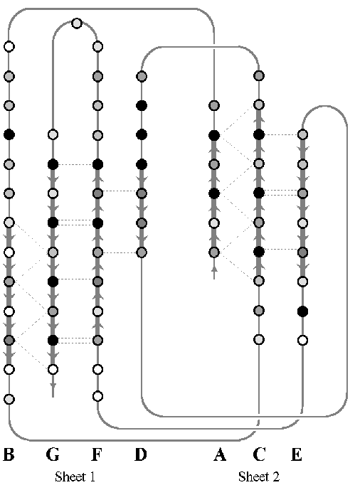
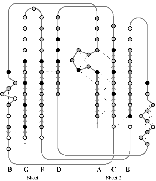
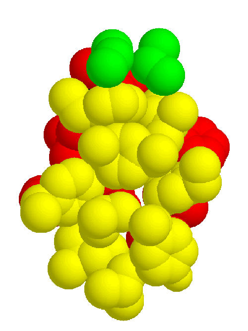
There are multi-domain and single domain cupredoxins. Only the family of single domain cupredoxins is considered here. There are seven types of cupredoxin for which a structure has been experimentally solved: plastocyanin [35], amicyanin [36], pseudoazurin[37], plantacyanin [38], azurin [39], rustacyanin [40], and stellacyanin [41].The cupredoxins are a superfamily of two-sheet beta sandwiches, of which the plastocyanin/azurin-like family comprises all of the monomeric proteins. The highest resolution structure available for each of the seven domains contained within the family are considered. Plastocyanin is used as a standard for the family, to which the others are compared. The members of the family are single copper (or blue) binding proteins involved in electron transport, particularly in systems of photosynthesis and respiration. Although it is a very diverse family (all sequences less than 20% identical), there is nevertheless a conserved beta-sheet sandwich, with a common core, and the strongly conserved ligand binding site. The two sheets are made up of seven parallel and anti-parallel strands, with a variable alpha-helix at one edge, and the binding site mostly atop one sheet. They occur mostly in plants but also in some bacteria.
Previous work has been carried out on the analysis of the structures of the cupredoxin family [42] but it differs significantly from the work presented here. Their approach is quite different to that here, and in addition to the monomeric cupredoxins they analyse the multi-domain cupredoxins which are not considered here. In particular they are concerned with a sequence alignment for the whole family. The work shown here is all novel; in particular the definition of the core of the family, the identification and characterisation of the key residues, analysis of the binding sites and sheet movements are all new.
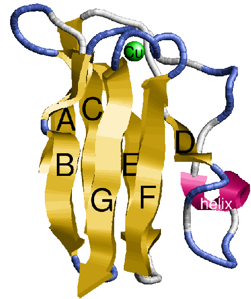
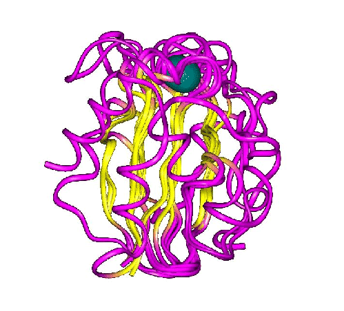
The basic structure in figure 2.1 is common to all, except for the alpha helix and loop regions which are variable. Although the two sheets are conserved amongst the structures, the positions of the sheets relative to each other may vary. There are two beta sheets with the strands labeled alphabetically from the N to C terminus, and a copper atom binding site supported by the sheets.
|
|
The first task was to calculate all of the backbone hydrogen bonds which join the strands into parallel and anti-parallel beta sheets. This was done for all seven structures, and diagrams were drawn detailing the bonds in a similar way to figures 2.3 and 2.4 (later). The pattern of hydrogen bonds identifies the strands in the two sheets and suggests an initial set of equivalent positions between structures. The conservation of hydrogen bonds also gives an initial suggestion as to the extent of conservation. Later on, figures 2.3 and 2.4 show the hydrogen bonds which are conserved between structures.
When comparing two hydrogen bond patterns, a spatial shift of two residues either up or down, in the plane of the sheet produces an alternative solution. As a consequence the hydrogen bond diagrams do not always give an unambiguous positional equivalence of strands, and the correct solution must be determined by doing three-dimensional superpositions.
Once the backbone hydrogen bond patterns have been used to suggest an initial structural alignment, full superpositions can be carried out. Figure 2.2 shows the result of full superpositions between three structures; the conserved strands are clearly aligned whereas the loops and helices are not. Plastocyanin was chosen as a `master' structure and the other six structures were each in turn aligned to it.
The procedure for structural alignment made use of a program called `PINQ' for three-dimensional analysis written by Arthur Lesk and is as follows. The superpositions were all pair-wise between plastocyanin and another. Although there is very little difference in the structures between strands in a sheet, there can be more variation in the relative position of the two sheets to each other (see the end of the section). The initial work on hydrogen bond patterns was used to define an equivalence of a few residues on each strand of a sheet between the two structures. These positions alone were used to fit the two structures to each other by minimising the r.m.s deviation between the backbone atoms. The region of each strand which was superposed was extended by attempting to include one more residue along the chain, then re-fitting the structures. Any residue position with c-alpha backbone atoms in the two structures deviating by more than three angstroms from each other was rejected, but a better fit meant that the new position was added to those already included in the structural alignment. In this way all strands were gradually extended at either end by adding one residue at a time until no more positions could be added without producing a c-alpha atom difference of more than three angstroms.
Once the two sheets of the structures had been independently aligned to their plastocyanin counterparts, the positions from both sheets were used to fit the whole structure minimising the r.m.s deviations of both sheets at once; this gave the final structural alignment. The results of the structural alignments are shown in table 2.1.
|
|
Once the pair-wise alignments have been made, a comparison of the regions of plastocyanin which align to the other structures can be used to find the regions which are common to all. This effectively gives the multiple structural alignment between all of the cupredoxins. The equivalent regions of all seven structures are listed here using the PDB residue numbering in the `ATOM' records:
It is possible to calculate the contacts made by residues in the protein, that is atoms of different residues whose distance apart is less than a specified threshold. Although contacts were mostly used to identify the residues involved in the binding site (see later), they were also used to help decide the alignment of strands of beta sheet between two structures when there was any uncertainty. Contacts between peptides in the tightly packed core of the structure tend to be conserved, and hence give information in addition to the hydrogen bonds.
The accessible surface area was calculated using PINQ for every residue aligned in the structural alignments. The accessible surface area is the area of the peptide which can make a van der Waals contact with the surface of a water molecule on the surface of the protein. The accessible surface area indicates which residues are on the surface of the protein and which are buried and to what extent. All of the analysis so far is brought together in figure 2.4 for the rustacyanin-stellacyanin sub-family, and in figure 2.3 for the superfamily including plastocyanin and the others. The hydrogen bonds, structurally conserved residues, secondary structure, contacts, and accessible surface area all go toward defining the common features of the family, and most importantly the inner core of the protein (see later).
|
|
The information gathered in the previous section is necessary to define the common core, which consists of the binding site and the inward-facing residues of the two sheets which support it. The part of the core of the cupredoxin family responsible for maintaining the fold is shown from different angles in figures 2.5, 2.6, and 2.7. The residues in the inner core of a protein are generally buried and pack tightly together. As a consequence there are very strong structural constraints on the residues in the core, and only a limited variation is possible without disrupting the fold of the protein and de-stabilising it. These evolutionary structural constraints are observable in the sequences of the proteins of the family; the residues identified in the core are strongly conserved, whereas the other regions can be extremely variable in sequence. The identification of these key residues in the core which are responsible for maintaining the fold constitute the minimum requirements of any member of the family. If the properties of these residues can be ascertained then this information is a very powerful and can be used to determine whether a sequence of unknown structure could be a member of the family, with key residues with the same properties, and the same conserved core, and hence overall three-dimensional structure, and ultimately the same (or related) function.
|
|
|
To investigate the properties of the residues in the core of the protein, additional sequences of unknown structure are used to provide more information. By aligning other sequences to those of known structure the possible variations in the residues in core positions can be observed. It was mentioned at the end of the last sub-section that the key residue information can be used to identify homologues, but it is still possible to detect some homologues using sequence information alone.
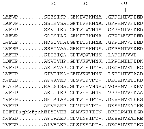
The sequence of each of the structures was compared to a non-redundant database[43]. Fasta[20] searches were performed using the sequence of each structure in the analysis individually. Sequences that were found by more than one of the searches were assigned to that with the strongest similarity. For each search, partial sequences were eliminated, then those remaining were aligned to the sequence of the structure used for the search using clustalw[44]. The result was seven sequence alignments of non-redundant homologues from a sequence database. The accurate structure-based sequence alignment of the seven proteins was used to align the seven alignments to each other, creating one large alignment of 84 sequences. This large alignment was carefully studied and adjusted using the results of the structural analysis to correct the alignment of the homologous sequences. Where necessary further investigation of the structures was carried out to solve specific uncertainties in the alignment. The final alignment is in the appendix.
The alignment of 84 sequences was analysed to see what variations occurred in the residues of the conserved core and binding site. The data referred to in the rest of this sub-section is in the appendix. The occurrence of every amino acid in each column was counted. From this the number of residues were added up of each of the types: surface, neutral, and buried. These types are simply defined by grouping the residues based on characteristics such as hydrophobicity and can be seen in the appendix. The same grouping as in the previous immunoglobulin work [34] was used.
A simple program was written to extract the salient features at each site based on the frequency at which the residues and types are observed. The result of the following residue analysis for the conserved positions in the large cupredoxin alignment is in the appendix. A score was calculated for every combination of residues, and for every combination of types (surface, neutral, or buried). The highest scoring combination of types and the top-scoring three amino acid combinations were displayed along with the percentage of all sequences satisfying the combination. The score for any given feature (combination of allowed residues or types) was calculated as the negative log odds probability of getting the observed frequency of the amino acids in the feature. The background distribution of amino acids was taken from the numbers observed in the whole alignment. Thus the program picks and scores the most significant features of any column in an alignment.
As an example the position corresponding to residue 14 in plastocyanin has 49 phenylalanine, 20 tryptophan, 7 tyrosine, and 1 aspartic acid residue in the alignment. It is obvious that a good score would be given to the feature ``phenylalanine or tryptophan'' , but the calculation shows that a better score is given to ``phenylalanine, tryptophan, or tyrosine'' and that a worse score is given to ``phenylalanine, tryptophan, tyrosine, or aspartic acid''. This might not be obvious by inspection.
Combining the structural and sequence analysis leads to the final characterisation of the family. Figures 2.8 and 2.9 show the structural and sequence determinants of the two beta sheets making up the proteins in the cupredoxin family. This information summarises and concludes the main part of the analysis.
|
|
In addition to the main part of the structure, the binding site is an important and well-conserved feature worthy of further examination.
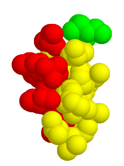
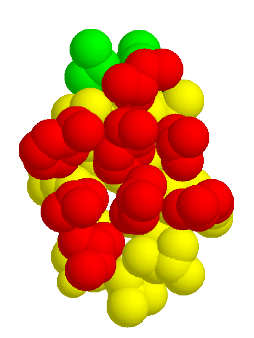
In plastocyanin the copper ligand is completely buried and has bonds with five residues, which form a tetrahedral shape. At the ends of strands G and F of sheet one there are a methionine and a cysteine which both form sulphur bonds with the copper. This is the base of the tetrahedron. Two histidines in loop regions form charged aromatic ring bonds. These are the sides of the tetrahedron. One of the histidines is in the mid-loop between the G and F strands of sheet 1, and the other in the loop between the C and D strands joining the two sheets. The second histidine has an important adjacent alanine residue preceding it which is involved in maintaining the position of the histidine. Following the second histidine is the fifth and final binding residue which is the weakest of the five and forms a bond via a backbone oxygen atom with the copper (fairly weakly at just less than four angstroms). The binding site of plastocyanin is shown in figure 2.10 and the binding sites of all of the other six structures in the analysis are in the appendix.
The binding sites of the other structures in the family follow the same pattern but the fifth bond with the backbone is often weaker. The fifth binding residue (glycine) is less conserved because it is the backbone which binds, putting less of a constraint on the residue which is a proline or a leucine in some other structures. The contribution of the fifth residue to the binding site would not be identifiable if it were not for the collective analysis of all structures showing that although it is very weak it is conserved. In fact the publications of the structures do not identify the backbone as being involved in the binding site at all. The greatest variation of the binding site is in stellacyanin where the cysteine in strand F is a glutamine which makes the site more exposed and flatter.
|
Table 2.2 shows the relative shifts of the sheets in the structures, compared to the positions of the sheets in plastocyanin (1plc).
|
The procedure for calculating the shifts is as follows. First the master structure (plastocyanin) is moved to a chosen orientation about the z-axis. Then the master structure is moved such that the backbone atoms of the conserved residues in the second sheet have a minimum r.m.s. deviation from the x-y plane. The master structure is then moved in the plane such that the centre of mass of the backbone atoms of conserved residues in the second sheet lies at the origin. The second structure which is to be compared to the master is then placed such that the backbone atoms of the conserved residues in the first sheets of both structures have a minimum r.m.s. deviation from each other. Finally the translations and rotations necessary to move the second sheet of the master structure to the position of the second sheet of the second structure are calculated.
The movements of the sheets relative to each other are large compared to the movements within sheets. This means that although there are very strong structural constraints holding the strands in their positions in the sheets, there is much less of a constraint on the whole sheets to move relative to each other.
Unlike the immunoglobulin variable domains which make use of the variability of their loops in their function, the cupredoxin family has a strong constraint on the binding site required to maintain the function of binding the copper atom for electron transport. To maintain the tetrahedral binding there is strong conservation of the residues in the loops which actually bind the copper atom. Residues in the loops surrounding the binding residues are also important to hold them in the right position and are also conserved. The binding site is supported by the rest of the structure. The binding site sits mainly atop sheet 1 consisting of residues in the loops between strands of the sheet. As a consequence the sheet supporting the binding site is also required to maintain the function, and hence the tight-packing, hydrophobic, inward-facing residues of the sheet have a limited number of allowed sequence variations. Although sheet 2 provides the other half of the sandwich and inward-facing residues of the buried core of the structure, it's only direct involvement in the binding site is the central strand C which leads into a loop joining sheet 1 which contains one of the binding residues. As a consequence, unlike in the immunoglobulins, there are fewer constraints on the sequence of sheet 2 whose position relative to sheet 1 and the binding site is variable.
This chapter describes the detailed structural analysis of the family of monodomain cupredoxins. The buried tightly packing core of the structure is defined. The key residues which are in the core and thus determine the fold of the protein are determined. The structurally constrained key residues have their characteristics determined which are required to maintain the structure of the protein common to the family.
The work in this chapter can be considered independently from the other chapters, but the structural viewpoint emerging from this detailed analysis of a single protein family, is carried through the other chapters, which move toward less detailed work on the broader set of all known structures.
Hidden Markov models (HMMs)[10,11,12] have more uses than those described in this thesis, most notably in speech recognition [45]. HMMs can be used to detect distant relationships between proteins based on their amino acid sequences, and this is what is described here. There are other applications within computational biology, such as recognition of trans-membrane helices [46], CpG islands, and signal peptides [47]. Some of the principles in this brief description also apply to other applications, but it is by no means general.
The model itself is not of primary interest and may be most easily thought of as a profile (in this case of a group of proteins) which embodies certain characteristics of protein sequences. What follows is a description of the model constructed from a set of sequences, whose function is to emit random sequences consistent with patterns of residues found in the sequences used to construct the model. The relevance of random sequence generation is not explained until the next sub-section.
The model is made up of states and transitions between these states. The most basic state is a match state, whose function is to emit a single amino acid residue. The state is usually more likely to emit some residues than others. The match state has a probability of emission for each amino acid, and the 20 probabilities sum to one. A linear chain of these states joined by transitions between them from one to the next is a very basic model which is capable of emitting a random sequence, with one residue emitted by each state.
Since in nature the sequences have different lengths additional states are needed. A delete state is a state which simply emits nothing. The transitions to and from this state may allow it to bypass an emission state.
There are also insert states which are effectively the same as emission states because they emit a single residue and have a probability for each one. These however appear between match states and have a transition from themselves to themselves allowing the insertion of one or more residues between two match states. Match states vary a great deal in their probabilities but insert states are usually more generic.
The architecture is the way in which the states are linked by transitions to make a complete model. See figure 3.1 drawn by Martin Madera.
|
There are two special states to begin and end the sequence. Not only are there emission probabilities in the insert and match states, but there are probabilities for all transitions between the states, making deletions and insertions more or less likely in different places. A sequence is generated by starting in the begin state, then following a transition to another state, where a residue may be emitted, then on to the next state and so on until the end state is reached. There are many possible paths through the model.
Random transitions through the model and emissions from the states are guided by the probabilities, and a sequence is generated. Since the output from the model is a sequence, the states are `hidden' because they cannot be seen by looking at the output sequence. The sequences generated will on average have the characteristics which the model embodies via the variation in transition and emission probabilities. If a hidden Markov model is designed to represent a group of proteins, then the sequences it emits should be potential members of the group (in reality these generated sequences are unlikely to be biologically functional).
The ability to generate sequences is of limited use, but the model lends itself to more useful applications.
The most important application for the work in this thesis is that of remote homology detection. Pair-wise sequence comparison methods ask the question ``are two sequences related or not?'', but this is limited since some related sequences have very little similarity[48]. Profile based methods ask the question ``given a group of related sequences, is another sequence related to that group?'' and are far more effective than pair-wise methods[32]. An HMM is such a profile representing a group of proteins.
It is possible to calculate the probability of a sequence having been generated by a model, and hence a score relating the sequence to the group represented by the HMM. A database of protein sequences can be searched by a model for members of the group by scoring all sequences in the database and selecting those with a significant score.
The detailed method by which the emission probability of a given sequence from the model is calculated is quite complicated, and two algorithms are widely used: the Viterbi algorithm calculates the probability of the sequence generated from the most likely path through the model and the forward algorithm calculates across all paths. Probabilities obtained in this way are actually a bad statistic in practice, so a null model is introduced to correct for sequence length. There are a variety of null models to choose from. A very simple null model would be a model of the same length with emission probabilities corresponding to the frequencies observed in nature, thus mimicking a random sequence with no preference. A better null model has the emission probabilities derived from the geometric mean of the probabilities in the model, thus reducing the importance given to similarity in sequence composition. Possibly the best null model is the reverse null model. This takes the reversed model as the null, simultaneously addressing the problems of sequence composition and low complexity sequence. Another advantage of the reverse null model is that it can be used to generate E-values (see later).
For more detailed information on scoring algorithms see `Biological sequence analysis' [49].
If a model is to represent a group of proteins, the emission and transition probabilities must be generated in such a way as to capture the characteristics of the group, for example figure 3.2. A model is generated from a multiple sequence alignment. The residues in the columns of the alignment are used to generate the match state probabilities, and the insertions and deletions in the alignment to generate the transition probabilities. Sequences in the alignment are weighted such that their contribution is related to their similarity. In this way if there are a large number of sequences with high similarity and a few with distant similarity the model will not be over-dominated by the numerous similar sequences.
|
The algorithm used to estimate the probabilities from the (weighted) amino-acid frequencies in the alignment is quite involved. Since the observed residues in the alignment only represent a sample of the possibilities, one would not want a zero probability for a residue which does not appear in the column of the alignment. This is avoided by mixing the observed residue frequencies with some fixed set of probabilities. These fixed sets are called Dirichlet distributions [29] and were obtained by examining the observed frequencies in a very large number of naturally occurring sequences to give a background probability (Dirichlet distribution). One final twist is that there is not just one Dirichlet distribution to use on a given column in the alignment; there is a set of Dirichlet distributions called a Dirichlet mixture (or library of priors) with different characteristics representing different residue types.
Also relevant to this thesis is the use of HMMs for sequence alignments. As was explained earlier, it is possible to calculate the most likely path through the model for a given sequence. This path gives an alignment to the model; every match state which the path goes through gives a residue of the sequence aligned to that segment (column) of the model, and insertion emissions fall unaligned between states, with delete states leaving a column in the alignment blank. This alignment alone is of limited interest, but if other sequences are also aligned to the model then this gives a pseudo-multiple alignment of sequences. It is not a true multiple alignment because the alignment of every sequence is unaffected by the others, however it is more than a collection of pair-wise alignments because the model to which they are aligned is a profile representing a group of sequences. Figure 3.1 shows the alignment of sequences in figure 3.2.
 |
Expectation values (E-values) are a general value not specific to HMM methods, but they are used extensively in this work. In theory E-values from any method should be comparable.
Since HMMs are a probabilistic method, statistically one expects occasional chance errors. E-values are the expectation of the number of errors per query. If an HMM is used to score a database of sequences (a query), then the expected number of sequences unrelated to the model (errors), which have the same score or better than any sequence, is given by its E-value. It is important to note that an E-value is only true in the context of the query, for example a query on a large database will have more errors than a query on a small database searched with the same model. E-values can be used to decide what error rate you are prepared to allow in your results, but they say nothing about the success rate.
The errors produced by HMM scores follow an extreme value distribution. One way of estimating E-values is to score the model against a large number of random sequences (assumed unrelated to the model, and therefore all errors) and plot the distribution. An extreme value distribution can be fitted to the results and used to estimate the E-values of scores produced by the model. Another approach is to score the reverse of the sequence as well as the sequence itself; this is the reverse null model mentioned earlier.
Since the reverse sequence has the same error distribution as the forward sequence, subtracting the reverse score from the forward score cancels out the component of `error' from the distribution. Both forward and reverse scores are expected to be drawn from the same Gumbel distribution which has two parameters, however the difference of two variables drawn from the same Gumbel distribution follows a simpler one-parameter distribution. It appears to be the case empirically that the parameter is the same for all models and equal to one, so the distribution of the differences in forward and reverse scores is known. The E-value can then be directly estimated from the query conditions (database size), without the need for ad hoc model calibration requiring the scoring of random sequences and fitting the distribution.
There are numerous methods for detecting homology between protein sequences, but they fall into two basic categories: pair-wise methods (such as Blast[21] and FASTA[20]) and profile methods. As mentioned earlier, HMMs are a profile method and although pair-wise methods are much faster, profile methods are able to detect much more distant relationships[32]. Probably the most commonly used profile method is Position Specific Iterative Blast (PSI-Blast)[28] which is comparable in performance (see later), but HMMs are also widely used for remote homology detection.
There are two commonly used software packages for using HMMs for protein homology detection: Sequence Alignment and Modeling system (SAM http://www.cse.ucsc.edu/research/compbio/sam.html) and HMMER (http://hmmer.wustl.edu). The two methods are examined in more detail later but a key point is that to build a model, a multiple sequence alignment of homologous proteins is required, and the SAM package includes a procedure for automatically generating them, whereas HMMER does not. This represents a significant advantage of the SAM package.
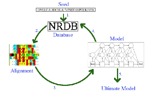
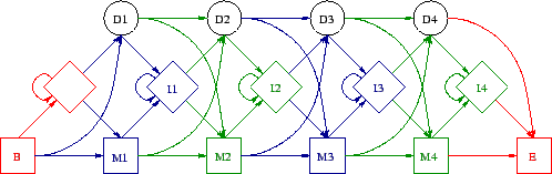
The SAM package comes with a procedure called `T98'[14] which was later improved and renamed `T99'. This procedure creates multiple alignments of homologous sequences for the purpose of model building. The procedure begins with a seed, which can be a single sequence or a set of sequences, aligned or not. The procedure then uses a large database of sequences from which to extract homologues by an iterative process to add to a growing alignment.
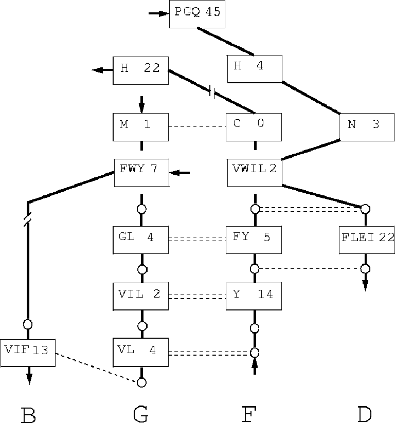
The default T98 procedure follows these steps (see figure 3.3):
Previous practice by the MRC bioinformatics group[50] and others[51] has been to build one HMM for each protein family or superfamily using an accurate alignment of the sequences of diverse family members. However, there are two problems with this approach: one practical and one theoretical. The practical problem is that producing accurate sequence alignments is not a trivial problem and for very diverse sequences requires expert human intervention. The theoretical problem is that it has not been demonstrated that using one model built from a good alignment of selected diverse sequences produces better results than using multiple models built from different single seed sequences and their homologues (as described above). To investigate this second problem various methods of modeling five chosen superfamilies were compared.
Five superfamilies were selected because detailed structural and sequence analyses were available, along with the expert knowledge acquired from the analysis (previous work, published[52] and unpublished). This provides both accurate structure-based hand built sequence alignments, and the means with which to verify the results of homology searches. The different models were built for each superfamily and searched against NRDB90, and then checked and compared. All of the models were built using the SAM T98 iterative procedure described above. The following four variations on the method were investigated:
|
The results are shown in table 3.2. The homology criteria were as follows: any hit with a `reverse' score lower (better) than -15 was taken as a homologue, hence the comparisons presented above depend on the scores produced by the different methods being roughly equivalent. This value (-15) was the score found to produce a 1% rate of errors per query when using T98 to score all of PDB versus PDB[32]. The `reverse' score is the forward score offset against the score of the sequence in reverse, which filters out low-complexity matches. The target sequences were checked by hand for false homologues using a combination of annotation, alignments, structural knowledge and further sequence searching. A small number of unannotated potential false homologues were found to be in the search results, and only a couple of certain false homologues. The immunoglobulins were not checked because the homologues were too many, and in the case of the flavodoxins the nitric oxide reductases were not counted as false because they are a well known case of sequence similarity between different proteins[53]. The results indicate that the use of multiple models where each starts with a single sequence produces the best results. When sequence alignments are used the addition of the constraints described in (2.) have little effect. The Cupredoxin hand alignment included only members of 1 of the 3 families within the superfamily and in this case procedure 2 did badly. The data also shows that there is some loss in performance using automatic alignments for seeding the T99 procedure, but not a great deal. Further analysis of this data (tables 3.3,3.4, and 3.5) shows that not only did the multiple models procedure (4) provide more hits but it found essentially everything found by the others.
|
|
|
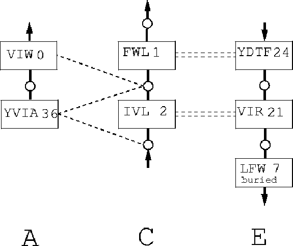
The multiple model method can be seen as modeling a family of proteins by several multiple overlapping models rather than one single model. Because a single model is too general to contain all of the features and variations in a family, the multiple models together can better represent more complex and diverse sequence variation. See figure 3.4 for a representation.
|
| Seed sequence | only this model | only other models | this and others | model sequences |
| 1plc | 1 | 59 | 46 | 49 |
| 1paz | 0 | 60 | 46 | 48 |
| 1aaj | 2 | 59 | 45 | 49 |
| 1aiz | 14 | 86 | 6 | 21 |
| 1rcy | 2 | 95 | 9 | 6 |
| 1jer | 0 | 69 | 37 | 39 |
| 2cbp | 1 | 68 | 37 | 40 |
| Seed sequence | only this model | only other models | this and others | model sequences |
| 256b | 2 | 20 | 0 | 21 |
| 2ccy | 20 | 2 | 0 | 4 |
| Seed sequence | only this model | only other models | this and others | model sequences |
| 5ull | 20 | 5 | 105 | 73 |
| 1ofv | 5 | 20 | 105 | 67 |
| Seed sequence | only this model | only other models | this and others | model sequences |
| 1bab | 0 | 77 | 428 | 419 |
| 1mbd | 0 | 55 | 450 | 442 |
| 1eca | 0 | 53 | 452 | 196 |
| 1lhl | 4 | 20 | 481 | 266 |
| 2lhb | 1 | 22 | 482 | 491 |
| 1mba | 0 | 13 | 492 | 329 |
| 1flp | 1 | 21 | 483 | 265 |
| 3sdh | 0 | 39 | 466 | 388 |
| 1hbg | 1 | 29 | 475 | 386 |
| 1ith | 0 | 53 | 452 | 215 |
| 1hlb | 0 | 25 | 480 | 440 |
| 1ash | 1 | 408 | 96 | 36 |
|
The complete breakdown of models is in table 3.6. The individual models in this procedure mostly found the same hits, which implies that a successful model built with T99 represents the family, and not the seed as is often misunderstood. This important point is discussed in more detail later. Some models were completely redundant with respect to others and some found outliers which the others did not find (see later for a more detailed analysis of model redundancy). These results solve the theoretical problem of whether one model or multiple models are most effective, and hence remove the need for solving the practical problem of accurately aligning distantly related sequences for the purpose of generating good hidden Markov models.
The examination of a small number of families was necessary because of the lack of good structure-based hand alignments, but when investigating the multiple models procedure further, it is possible to carry out large scale assessments which will give more accurate results.
The test procedure used in the previous section relied on a hand analysis of the results to verify the success or failure of a model. This is far too time consuming to carry out on a large scale, or to repeat for many conditions. It is desirable to increase the size of the data set which tests are carried out on (to make the results more significant), and to find a data set which spans more diverse families of proteins (to make the results more universal). To do this a large set of protein sequences is needed, with reliable independent family information. The SCOP[6] database provides such a set.
The Structural Classification of Proteins database contains all proteins of known structure with coordinates deposited in the PDB[54], and is usually kept up to date to within six months. SCOP is a domain based classification where genes may be comprised of one or more SCOP structural domains. A SCOP domain is defined as a minimum evolutionary unit. These are globular units, but unlike other databases, combinations of globular units are only separated if they are observed separately elsewhere in nature, i.e. in combination with different partners or in isolation. This means that some pairs (or more) of globular units are classified as a single domain because they are only observed together, and hence the pair (or more) is the minimum evolutionary unit.
SCOP is a hierarchical classification with several levels:
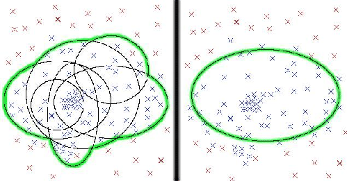
As was alluded to above, the test is carried out at the superfamily level. Since the structural and functional evidence used to classify the domains is able to link more remotely related domains than sequence information alone, the ability of sequence methods to detect SCOP superfamily relationships is a sufficiently hard test. The test could be used to assess the performance of any method, but the T99 method is used as an example in this description.
The sequences of all of the SCOP domains filtered to 95% sequence identity (to eliminate redundancy) were used as seeds for the T99 procedure, creating an HMM for each one. These models are scored against the sequence database from which they were built. The SCOP classification is then used to decide for every hit made by every model whether it is a true or a false homologue. A model built from any given seed is supposed to represent the superfamily which the seed belongs to, and any hit to a sequence in the same superfamily is considered a true hit. See figure 3.5 for a diagram of the test procedure.
|
This test has been used in previous work [48,32]. The same test was used to compare profile and pair-wise methods as mentioned above. The data produced by the test carried out on the HMMs provides the framework for the analysis in following sections.
When considering the hits made by any method on the SCOP test some exceptions to the superfamily classification should be taken into account. Since the classification is conservative it is possible that some superfamilies are classified apart when there could be a relationship between them. This can be dealt with by allowing hits outside the superfamily but within the same fold to be ambiguous, and are not taken as either true or false. There are a few known inter-superfamily relationships which are considered acceptable, most notably amongst TIM barrels[55], and between Rossmann folds[56].
The test described above has been used to investigate various aspects of the behaviour of HMMs built with the T99 procedure.
The early tests were carried out on SCOP version 1.48, using all domain sequences filtered to 95% sequence identity, producing 4951 models. The sequences were obtained from the ASTRAL database[57], which is discussed in more detail later. The default T99 procedure was used with no modifications.
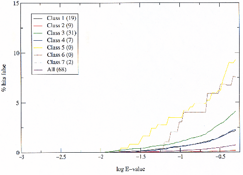
The first thing examined was the ratio of true to false hits for any given E-value threshold (figure 3.6). The different SCOP classes were compared and it was found that their behaviour differed significantly. The same results were calculated taking hits to the same fold but a different superfamily as false, rather than ambiguous as described above. This showed no qualitative difference, and only a very minor quantitative change. This means that differences in fold variations in the different classes are not responsible for the differing results in figure 3.6.
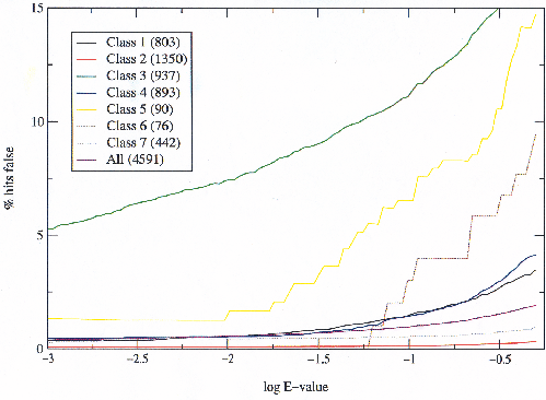
| Class | Description |
| 1 | All alpha proteins |
| 2 | All beta proteins |
| 3 | Alpha and beta proteins (a/b) |
| 4 | Alpha and beta proteins (a+b) |
| 5 | Multi-domain proteins (alpha and beta) |
| 6 | Membrane and cell surface proteins and peptides |
| 7 | Small proteins |
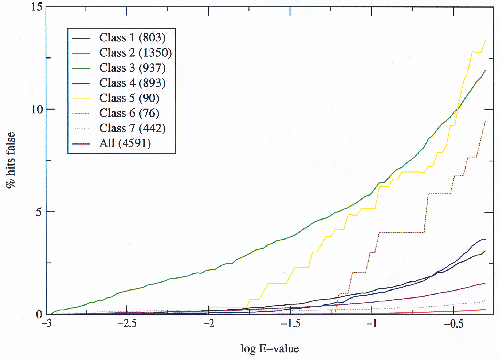
Since the classes vary a great deal in size, different sized sub-sets of the SCOP domains were examined (figure 3.7). The sub-sets were created by filtering the seeds to different percentages of sequence identity. The classes have different numbers of folds and superfamilies; they are not homogeneous with many superfamilies over-represented, under-represented, or not yet represented at all by known structures.
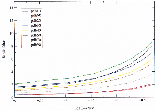
|
There is an obvious trend in the graph showing an increase in the ratio of false hits to true as the set size decreases. This is what one would expect as at lower percentage sequence identity the closer homologues which are easier to detect are fewer with respect to the more distant ones. The behaviour is unclear below 40% sequence identity because below this level, percentage sequence identity is a very poor measure of similarity.
To observe the effect of size alone, the same experiment was carried out except the seeds were filtered randomly to produce sets the same size as those filtered on percentage sequence identity (figure 3.8). It is clear from these results that there is no significant difference between the sets of different sizes, and so this cannot explain the observed differences between SCOP classes.
|
From the graphs above it can be seen that class 3 has by far the greatest ratio of false hits to true hits, so an experiment was devised to test the hypothesis that this is an artifact of classification. If for some reason proteins in class 3 which are related have been classified in different folds (the treatment of same-fold hits as ambiguous rules out merely trans-superfamily relationships), then these can be detected by low-scoring (good) inter-superfamily relationships. Any inter-superfamily hits below an E-value threshold of 0.001 define an `allowed' inter-superfamily relationship. These relationships then become true hits rather than false hits.
|
Figure 3.9 shows that the difference between class 3 and the others is due to inter-superfamily relationships which are being detected by the HMMs, which may be true relationships or errors in the HMMs. Classes 5 and 6 still produce more false hits to true hits than the others, but they are both quite small and the data is insufficient to draw conclusions from as can be seen by the `stepping' nature of the graph. What is also interesting is that relatively few inter-superfamily relationships are detected below 0.001 and that they appear to account for most of the false hits. To confirm that the improvement observed in class 3 by allowing certain relationships is across all scores, and is not merely explained by the exclusion of false hits below 0.001, the same graph was plotted simply making all hits below 0.001 true (figure 3.10).
|
Although the errors are reduced by considering all hits below an E-value of 0.001 as true, they only account for a partial contribution and the same differences as in figure 3.6 between classes are observed. It is thus safe to conclude that the differences between classes are due to discrepancies between the SCOP classification and the relationships detected by the HMMs, and that for some reason there are many more of these in class 3 than any other. Later on it is discussed whether these are failures of the HMMs or genuine relationships.
Since an E-value of 0.001 as a threshold is a somewhat arbitrary but reasonable value, the number of inter-superfamily relationships detected by the HMMs was plotted for a range of E-values to investigate what a suitable threshold might be (figure 3.11).
|
Most classes seem to detect a similar number of relationships (although class 3 has by far the greatest number of hits between them), with the exception of class 4 which detects far fewer. This is still unexplained. Examining the two extremes of the graph shows that at very high E-values relationships increase linearly implying totally random behaviour, and at very low E-values the number of relationships is almost constant implying a fixed number of non-random relationships.
To optimise a model library assembled from models such as have been created for the test, it is desirous to eliminate as many false hits as possible by removing models which are the cause of the false hits, yet at the same time keeping as many models as possible. To look at this issue the proportion of models making false hits was plotted for different E-value thresholds (figure 3.12). This is another approach to the same question addressed in the previous graph.
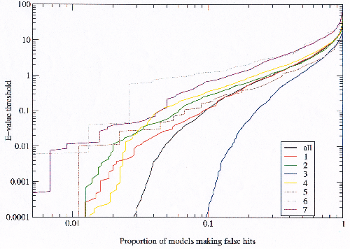
|
A detailed analysis of this data revealed a change in behaviour at some point in all of the curves. This change in behaviour can also be observed in the previous graph but is far less marked. The observation of this change in behaviour lead to an important conclusion which explains all of the data presented in this section. In retrospect it is obvious and the reader may have already been guided to the same conclusion, but the implication is very important for the work which follows.
Errors observed in HMMs are the result of two very distinct causes:
The point at which the change in behaviour was observed in the previous graphs was used as a threshold to identify models which had errors in them from the building process. This amounted to 4% of all models, and these 187 models were found to be producing 90% of the false hits. As mentioned earlier these `false' hits could be occurring for two reasons: either genuine inter-superfamily relationships are being detected, or the model has been poisoned during the model-building stage (I call these bad models). On close examination of the 187 models roughly half turned out to be bad models. The other half were explained by reasonable inter-superfamily relationships, a large proportion of which were Rossmann-like folds in class 3 with very distant similarities. There are some Rossmann folds which are obviously related and these were mentioned in the description of the test, but there are many more less obvious relationships which are plausible. This explains the observation of differences between class 3 and the others.
Comparing the errors produced by the model library before and after the bad models are excluded shows that the data fits the theoretical value predicted by the E-value better afterward than before, especially in the critical region (figures 3.13 and 3.14). At the bottom of the graph of the modified library no scoring errors are observed where there should be some; this is an artifact of using the E-value to select the bad models, and ideally an independent measure would be preferable. This result supports the explanation of scoring errors and model-building errors, with a small number of bad models generating most of the errors.
|
|
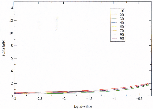
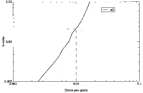
Since there is some discrepancy between the theoretical E-value and the observed errors per query it is possible to choose an E-value threshold which corresponds to the desired real error rate. Figure 3.15 is focused on the critical region of the modified library, and shows that the theoretical E-value is very close to the observed error rate.
|
A comparison was made to another method for assigning structural domains to protein sequences which has previously been shown to perform well[58].
Sequence homology is distributive, so that if two sequences `a' and `b' are related, and if `b' and `c' are also related, we may infer that `a' and `c' are related. It may be that we are only able to detect homology between `a' and `b' and between `b' and `c'. In this case we say that `b' is an intermediate sequence for detecting homology between `a' and `c'. This is a powerful technique as very distant relationships can be detected via a number of intermediates.
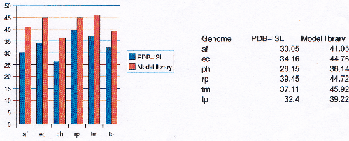
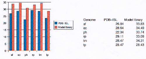
The Protein Data Bank Intermediate Sequence Library (PDB-ISL) is a library of sequences homologous to proteins in the PDB which can be used as intermediates for detecting remote homologues to proteins of known structure. The intermediates were found using PSI-Blast[28], and the performance of PDB-ISL is comparable to PSI-Blast alone, the advantage being that PDB-ISL is faster to search and hence applicable on a genomic scale. More information on PDB-ISL can be obtained from [58].
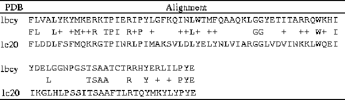
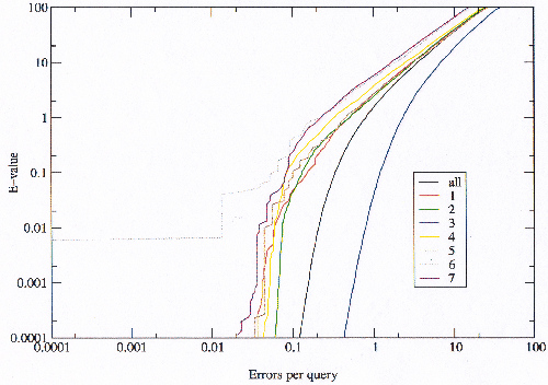
Work by Jong Park and Sarah Teichmann used PDB-ISL to assign structural domains to 6 complete genomes, so the model library was also used to carry out assignments to the same genomes so that the coverage could be compared. The results (figures 3.16 and 3.17) show that a significant improvement in coverage has been obtained over PDB-ISL. Both methods aim to achieve an error rate of less than 1%, but this can only be verified on PDB sequences.
|
|
Up to this point the SAM T99 procedure had only been used in its default mode of operation, and it was known that some options were sub-optimal (personal communication with the SAM authors). The T99 procedure was designed to be carried out as individual searches (rather than to create a search-able library), and so the default parameters were set to allow completion of model building in a reasonable amount of time. It is possible however in the context of building a model library, to use more computationally expensive and time-consuming parameters which might perform better. Since the cost of searching the model library is fixed by the number of models (and strictly speaking the number of segments in the models), then using more costly model building parameters only causes a large one-off computational expense, the benefits of which can be reaped repeatedly at no further cost by searching the library.
Some model building parameters were investigated in an attempt to improve the quality of the model library. These tests were carried out on SCOP version 1.50, using sequences filtered to 95% sequence identity.
There are a large number of options and parameters which can be altered in the SAM T99 procedure, most of which are documented in the SAM manual (http://www.cse.ucsc.edu/research/compbio/papers/sam_doc/sam_doc.html). The parameters which were varied in the tests were:
The effects of a basic set of five variations was chosen as a guide to the best method for building the final set of models. For each set of parameters a model library was built and scored against the sequences as described above. The five model libraries were built as follows:
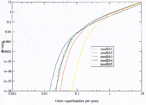
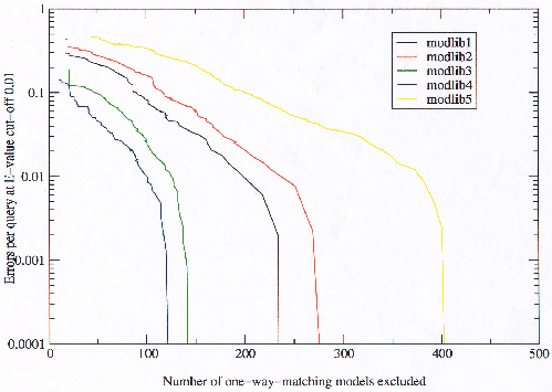
First the results from scoring all five model libraries will be examined in detail to gain an understanding of the behaviour of the model libraries (labeled modlib1 to modlib5). When the behaviour is clearly understood, the implications the results have to the various model building parameters will be discussed.
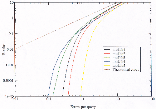
The number of true hits against false hits reveals (at the extreme) the possible number of relationships which a model library is able to detect, and hence the maximum potential of the model library were it possible to eliminate the false hits. Figure 3.18 shows that modlib5 has the most potential and modlib4 the least. It is not possible to see from figure 3.18 which is the best model library as it stands because it goes to the extreme of false hits.
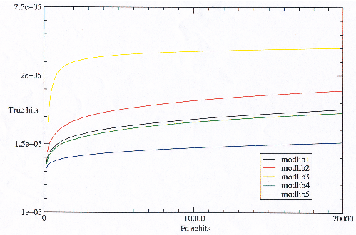
|
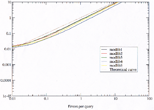
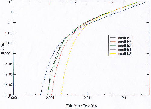
Figure 3.19 reveals that in the area of low error the situation is reversed with the model libraries with the most potential performing worse than those with the least potential, with the possible exception of modlib3 and modlib4, where modlib4 appears to be always better than modlib3. This trend is observed throughout the results. Figure 3.19 also shows that the order reverses toward very high E-values (in agreement with figure 3.18). Plotting only the true homologues against E-value (not shown), shows that the model libraries with the most potential find more true homologues at lower E-values, implying that they must also be finding proportionately more false homologues as well.
|
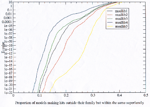
Comparing the observed error rate to the expected error rate (E-value) confirms that the model libraries with more potential find more errors at any given E-value (shown later in figure 3.25). This does not reveal anything about the nature of the errors, but figure 3.20 shows that not only are the models with more potential finding more errors, but they are finding these errors in a larger number of superfamilies. It would be possible that the models with more potential were merely finding more of the same errors but this is not the case.
|
By plotting the proportion of models in a given model library which make at least one error (figure 3.21) it is clear that the increase in errors in model libraries with more potential is not coming from the bad models finding more errors, but is caused by more models in the library being bad. This is especially true for modlib5 which has markedly more potential than the others.
|
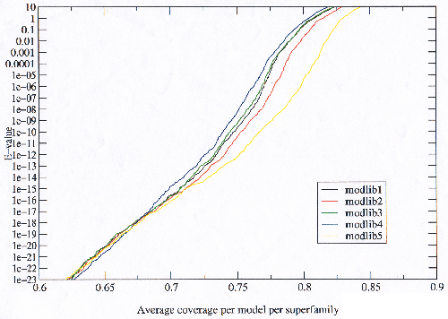
In the same way that it is possible that the bad models in the model libraries with more potential getting increased false hits could have been responsible for the observed error rates in figure 3.25, it is possible that the increased true hits be due to improving the best models, or models for superfamilies with the most members. Improving a model which is a member of a small superfamily will not increase the true hits a great deal whereas slightly improving a model in a large superfamily will make a larger difference. One measure of the quality of a model is whether it not only finds the closer homologues within its own family, but manages to find the more distant homologues in other families within the same superfamily. Figure 3.22 shows that in the model libraries with increased potential, the models are on average more general and closer to representing the superfamily than models in the other model libraries.
|
The coverage which a model library achieves is the ultimate goal, but counting the true homologues and dividing by the maximum possible number will give a result almost entirely dominated by the largest superfamilies since the possible true homologues is the square of the size of the superfamily. This is compounded by the fact that there is a very uneven distribution of sizes of superfamilies. Even after sequence filtering to 95% there are 526 members of the Immunoglobulin superfamily in the current (1.55) SCOP release, 71 members of the globin superfamily which is the next largest, and many superfamilies with only a single member. To normalise for superfamily size the average coverage per model per superfamily was plotted in figure 3.23. It was necessary to exclude singleton superfamilies from this because they have no possible true homologues. It is clear from the figure that the improvements in coverage observed in the model libraries with more potential are across all models which is very important when considering that sequences of unknown structure searched against a model library will not follow the biases in the PDB. This result means that the observed improvements are general and are likely to extend to genome sequences.
|
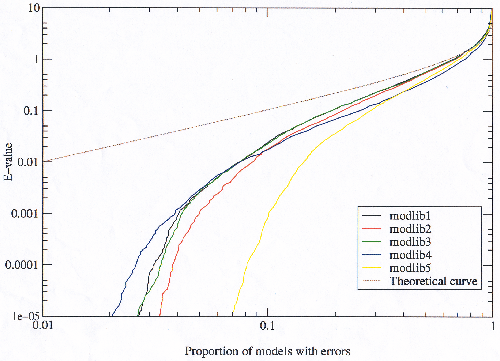
As explained in the previous section errors occur either at the model building stage or at the model scoring stage. What the results in this section have shown up to this point is that improved models can be built (those previously referred to as having more potential), but that the number of those models which will be bad models causing errors will increase. To examine the number of models which would be excluded from each library to give a required error per query rate (for a given E-value threshold), models were removed from the model libraries one by one in order of most errors, and the errors per query calculated for the new library. The results are plotted in figure 3.24. In the previous section it was observed that approximately half of the models appearing to cause errors were actually detecting genuine relationships. To take this into account, those models which made hits to another superfamily which also made hits to the first superfamily were not considered `bad', assuming that the chances of unrelated superfamilies both hitting each other are relatively small.
|
The same qualitative results were obtained at different E-value thresholds, and also plotting against straight E-value rather than observed error per query yielded the same result. The conclusion is that to achieve an observed error rate equal to the expected error rate only approximately 100-400 models need be excluded. It is also interesting that the curves all become very steeply descending, with the observed errors dropping off almost completely at some fixed (for each library) number of models. This confirms the theory of model building errors accounting for most false hits, and indicates that it is possible to detect and remove these bad models.
The results to this point indicate that it is possible to alter the model building procedure such that the models are more general and more closely represent a superfamily, finding more true hits achieving a greater coverage. This gain however is at an increased risk of generating a bad model, so a greater proportion of models built turn out to be bad. It appears to be possible to detect the bad models and remove them.
Finally the error rate was compared before (figure 3.25) and after (figure 3.26) bad models were detected and removed. These graphs show that although there are quite different error rates observed for different model libraries before bad models are removed, after the bad models are removed, the error rates are all the same. Further to that the observed error rates are very close to the theoretical expected error rates predicted by the E-values. The conclusion is that the optimal procedure is to build the model library with the most potential possible, and then to detect and remove bad models. The resulting library produces no more errors than the worst model library yet has a much improved coverage.
It was generally found that variations in the first three parameters (number of iterations, E-value thresholds, and size of culled set) described at the very beginning of this sub-section could have the effect of creating `looser' models which are more general and find more true homologues, but also increase the risk of making a bad model. `Tightening' the parameters made it possible to reduce the number of badly built models, but also the coverage. This can be attributed to the fact that `looser' parameters include more information in the models but increase the risk of including incorrect information during the iterative process, which leads to bad models. The more iterations which are used, and the larger the culled set, the more computationally expensive the model building becomes. Once again; an expensive procedure is affordable if it is only to be carried out once, because the models can be used again and again at no further cost. The changes in the other two parameters (prior library and final model building script) are of no extra cost. Using model-building script `W0.5' and prior library `recode3.20.comp' were found to be improvements on the defaults from work carried out by the SAM authors, which this work confirms. Tightening the threshold in the final iteration (also suggested by the SAM authors) reduces the number of bad models but does little or nothing to improve the ratio of true to false hits. For an automatic procedure this is very desirable, but in the case of the SUPERFAMILY model library which has bad models re-built by hand (see later chapters), doing this reduces the ratio of true to false hits.
Free Insertion Modules (FIMs) can be put between any two segments of a model allowing the free insertion of any sequence of any length. This amounts to a zero gap penalty for a specific position, and means that the score given to a sequence is unaffected by any number of residues inserted at the point of the FIM. FIMs are added to the beginning and end of the model when using local scoring, this allows the model to freely match any part of a sequence.
As described earlier SCOP classifies structural domains and many proteins consist of more than one domain especially in higher organisms. The nature of the evolutionary process of recombination is such that the basic units of domains get assembled in different combinations to form multi-domain proteins. Because the recombination occurs at the sequence level, often a domain is inserted within another domain's sequence but the protein still folds into the same three-dimensional structural units. An example of this is figure 3.27 showing two structural domains with one sequentially inserted in the other.
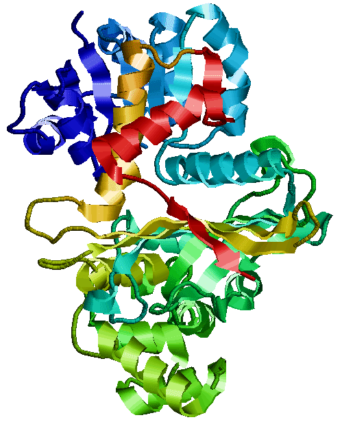
|
When building an HMM for a domain which may have another domain inserted in it, it may be desirable to put a FIM into the model at the point where the inserted domain can occur. This means that a sequence being scored against the model will not be penalised for an inserted domain at the point of the FIM.
Two ways of inserting FIMs were investigated. Firstly the FIMs were put into the ready-built models. The second method was to specify the position of the FIM in the seed sequence, so that the FIM is used throughout the iterative T99 process, affecting not only the final model, but the collection and alignment of homologues from which the model is built. All of the seeds with an inserted domain were collected and the unaltered model plus two different FIM models (described above) were scored against all of SCOP (filtered to 95% sequence identity). The success of the three methods were compared in figure 3.28.
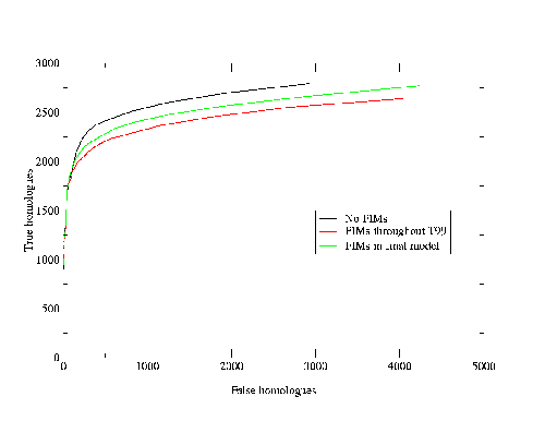
|
It is clear from the results that FIMs actually decrease performance, slightly more so if used throughout the T99 process. Examining the probabilities of models without FIMs revealed that the match-to-insert and insert-to-insert transition probabilities were extraordinarily high at one position in the vicinity of the possible inserted domain. This is very similar to a FIM, yet not allowing completely free insertion, the penalty instead being very low. This has happened because the sequence alignment produced by the T99 procedure includes large unaligned insertions in the point at which inserted domains are expected, and so the transition probabilities in the model were estimated accordingly. This means that homologues to the model are likely to be correctly aligned and scored around the inserted domains. The probable reason why the models without explicit FIMs perform better is that a very small penalty is better than none, only penalising the insertions when they become overly long. Another advantage in having some penalty (however small) is that in multi-domain proteins with homologous domains with a possible insertion, there is a lower chance of a model hitting two parts from different domains.
The redundancy of models is of interest because too little redundancy in a model library implies incompleteness; the model library would certainly be improved by increasing its size. Too great a redundancy in a model library implies that it could be reduced in size without loss of performance, and that perhaps the wrong criteria are being used to select the models to be created.
Once a model library has been constructed it may be examined and filtered for redundancy. Since the redundancy of the seeds of the models is only indirectly linked to the percentage sequence identity of the models other measures of similarity must be introduced. Two measures of redundancy from one model to another are defined:
The results are plotted in a scatter plot in figure 3.29. Although no two models in the library have exactly the same state and transition probabilities, under the two criteria defined above, 30% of the models were found to be 100% redundant on both counts. The covariance between the percentage sequence identity of the seed, model-building sequences, and genome sequence hits shows that there is no significant correlation of the sequence identity between model seeds and the sequence identity between genome hits made by the models (r=0.135). What this means is that sequence identity of the seeds of models is a very poor measure of similarity. Only 58% of models score their seed sequence higher than any other seed sequence, and only 33% score their seed higher than any sequence in the completed genomes. This means that a model really does represent its superfamily first and foremost, and not its seed sequence as must not be misunderstood.
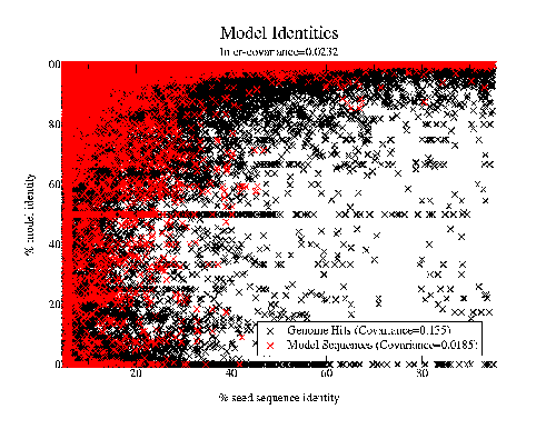
|
Studies on the effect of using models built from seeds filtered to different percentages of sequence identity showed that there is a strong fall off in the coverage achieved, beginning when using seeds filtered to 40% identity, and falling steadily from 30% and below (figure 3.30). Since reducing the library from 95% to 40% only gives a reduction of 1/3 in the computational cost, and some performance is lost (e.g. 50 assignments for an average-sized bacterial genome), the seeds filtered to 95% are still used. In fact, the main advantage in using the larger library is an improvement in the quality of the assignments, rather than an increase in coverage, i.e. better scores and better domain boundary definitions are given by models that would have been excluded by seed filtering.
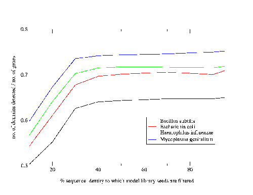
|
The work in this chapter forms the foundation of this thesis and expresses some important ideas:
This chapter also investigates many other important aspects of HMM behaviour and model library construction.
A library of models was built representing all proteins of known structure. This library of models is the basis of the SUPERFAMILY database described later. This chapter describes in some detail the construction of the library:
The SAM T99 procedure was used to build models from single seed sequences. These models were examined in the context of the SCOP classification and many models rebuilt. Changes were also made to SCOP (by the SCOP authors) in cases where discrepancies revealed errors.
Files in the ASTRAL database [57] provide sequences corresponding to the SCOP domain definitions and are derived from the SEQRES entries in PDB[54] files. Domains which are non-contiguous in sequence, i.e. parts of the domain separated by the insertion of another domain, are treated as a whole. Their sequences are marked with separators between the fragments representing regions belonging to other domains. All PDB entries with sequences shorter than 20 residues, or with poor quality or no sequence information are omitted. ASTRAL also has available sequence files filtered to different levels of residue identity. When filtering on sequence identity the ASTRAL files use the SPACI scores[57] to choose which sequence to reject. The SPACI scores are a measure of the quality of the solved structure, so the filtered files should contain the best examples of structures in the PDB. The ASTRAL entries are generated entirely automatically and hence have a small number of documented errors in the database.
The sequences which are used for the work presented here are generated from the ASTRAL sequences filtered to 95% identity yet differ in the following ways:
Some domains are split and therefore appear as more than one chain in the structure. These belong to the same gene, and should be considered together as they are part of the same functional and evolutionary unit. There have been cases where they do not belong to the same gene, for example if a histidine tag or ligand has been included in the domain definition. In these cases either the domain definition is altered in SCOP or the part is just removed from the SUPERFAMILY sequence. In the ASTRAL files all chains have separate entries and therefore the complete genetic domain split into more than one chain belonging to the same gene are not together. In the most recent release of the ASTRAL files genetic domains are available, but this recent addition was not available at the time of this work. It should also be noted that many errors in SCOP detected by this work have been fixed, so the new ASTRAL genetic domains are very similar to the SUPERFAMILY sequences now.
To generate the SUPERFAMILY sequences the domains split across chains were joined into single genetic domains. To do this the ordering must be obtained. This was done by searching NRDB and NRDB90[43] for very close homologues to the separate chain sequences. The genetic ordering was then derived from sequences which contained very close homology to all parts of the whole domain. The possibility of tandem repeats confusing the order was considered and only sequences containing all parts the same number of times in the same order were used. It was found that most sequences had homologues with 100% sequence identity giving the ordering, and almost all had sequences over 90% identical. There were a few problems which were adjusted by hand, for example with cyclically permuted sequences.
Once all of the models had been built from the sequence seeds described above, they were all scored against all of the seed sequences. Any model hitting a sequence from a superfamily other than its own was examined as a potential bad model. By examining the structures involved these discrepancies with the SCOP classification were explained, and some were found to be errors in SCOP.
In SCOP there are some known relationships between superfamilies which are documented. This accounts for the majority of inter-superfamily relationships found by the HMMs. Most notable of these are the NAD(P) Rossmann domains and the FAD/NAD(P), and nucleotide binding Rossmann-like domains (see SCOP annotation). There were many relationships detected between these two folds and a few others such as the N-terminal of MurD superfamily[56]. In fact several superfamilies in the Alpha and beta proteins (a/b) class in SCOP are distantly similar to Rossmann domains. The TIM barrel fold also has relationships between different superfamilies[55].
As described in the previous chapter SCOP domains may consist of more than one globular unit. Sometimes dimers are classified as a single domain, and sometimes as two separate domains. Some inconsistencies across superfamilies were detected where one member had been split into separate domains and another not. These have subsequently been altered in SCOP as a result, unless some explanation already exists, for example with 19hc which has an extra heme-binding site in the domain interface [59].
It is worth noting that the EF hands can be occur in two or four unit domains [60], and are classified together. In this case no attempts were made to make the domain definitions consistent in number of sub-units.
A problem occurs when the domain boundary definitions vary slightly from one protein to another , in these cases they can be made consistent in the sequence files. 1qtm (residues 423-447) and 1kfs (residues 519-544) show an example of this; there is a 6-turn alpha-helix which belongs to one domain in one definition, and the other domain in the other definition. These domain boundaries have subsequently been re-classified in SCOP.
A further cause is when two proteins have different domain boundaries which cause the parts to be classified differently. In the case of 1hfe (chain `s'),1feh (residues 520-574 chain `a') which are Fe-only hydrogenases a fragment is classified differently when it is a separate chain and when it is part of the main domain. In the case of 1qax (residues 4-108 chain `a') and 1dqa (residues 462-586 chain `a') a section which forms part of a domain is classified as part of another domain when the rest of its domain is not present. This has subsequently been re-defined in a consistent manner in SCOP.
Members of SCOP superfamilies are classified according to whether, in the light of the currently known structural sequence and functional evidence, they possess a common evolutionary ancestor. Use of this evidence is conservative in that proteins, for which evidence of an evolutionary relationship is not strong, are placed in same fold category but as separate superfamilies. This means that some models may well collect sequences that allow them to detect relationships between different superfamilies that go beyond that available from the current structural, sequence, and functional evidence. This is particularly true for TIM barrel superfamilies[55]. Also 1c20 and 1bmy (ARID-like domains) have sequence homology but were classified separately in SCOP (table 4.1). They have subsequently been re-classified.
A rare example mis-classification in SCOP is of 1zrn and 1ek1 (HAD-like proteins) which match each other and superimpose over 100 residues to within 1.655 angstroms r.m.s. deviation, indicating that they are clearly related structures (figure 4.1), and have subsequently been re-classified in SCOP. In SCOP 1.53 there was an immunoglobulin incorrectly classified as a fibronectin domain. As a result of this being detected it was re-classified in SCOP 1.55.
There are domains with local structural similarities which are detected by the models but the overall domain structure is different. 1b0p and 1fum (figures 4.2 and 4.3) have an interesting identical discontinuous structural motif, but the rest of the domain does not even share the same secondary structure, one being all alpha and the other being mostly beta.
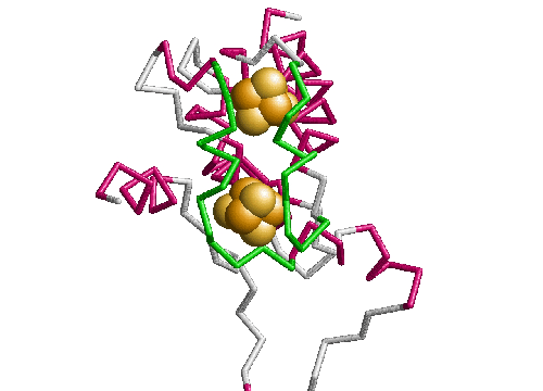
|
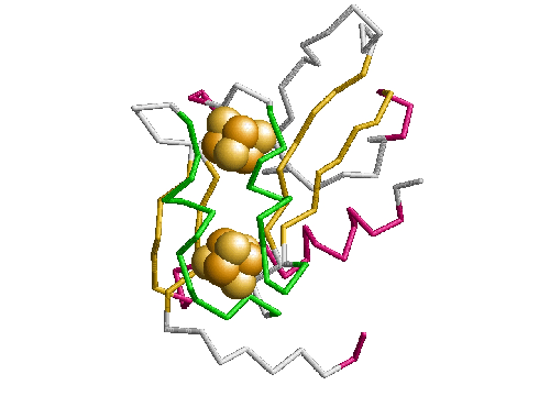
|
1psd (residues 108-295 on chain 'a' form a Rossmann domain) and 1b6r (residues 1-78 chain 'a' form a Biotin carboxylase N-terminal domain-like domain) superimpose 35 residues to within 1.14 angstroms, but the rest of the structure does not superimpose at all (figure 4.4).
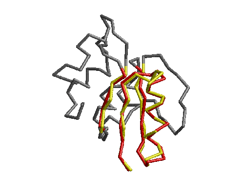
|
Of the models examined only a small fraction can be explained by genuine structural relationships as described in the previous section. This section examines the reasons why bad models are being built. It also describes how these problems were solved. In the previous chapter models were removed from the library if they are found to be bad. What is actually done for the model library is that bad models are re-built so that they are not bad. To do this properly it is necessary not only to identify the bad models but to know the reason for the error. Every bad model is inspected by hand and the cause for the problem identified and fixed. Since there are relatively few bad models (approximately 250) it is possible to do this although it is a lot of work.
There are cases where there is a simple disagreement between the SCOP classification and the homology suggested by the scores due to scoring errors (natural statistical fluctuations) and are not caused by badly built models. For example 1sig (sigma70 subunit fragment from RNA polymerase) and 2fb4 (Immunoglobulin), have 16 residues which align almost identically yet the structures are unrelated. The section in question is beta-sheet in one structure and helical in the other (figure 4.5). These are inevitable and models producing these are not considered bad.
The criteria for selection of bad models is quite strict and as a consequence some of the supposedly bad models appear so due to scoring errors. It is necessary to inspect and make a judgment on each of these. If a model has only one or two very low scoring (higher E-value than 0.001) hits with no obvious explanation then it is assumed to be a scoring error. Of course some of these may be due to model building errors but since they are producing such low scores keeping them will not have a great affect on the model library.
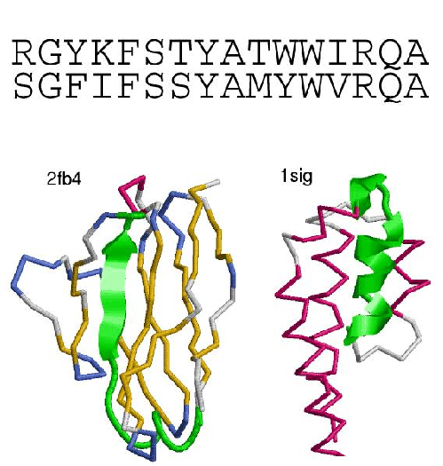
|
As described in the previous chapter the parameters chosen to use in the model building process affect how loose (general) or tight (specific) the model is. With the looser parameters the chance of poisoning the model during the iterative procedure with unrelated sequences is higher than for tighter parameters. By rebuilding many bad models with tighter parameters they simply don't get poisoned and hence become acceptable. Since the iterative process amplifies the effect of one poisonous sequence, a slight change in the parameters can cause a radical change in the final model if that change causes the one borderline poisonous sequence not to be accepted.
A common cause of problems is due to multi-domain proteins which have similar (e.g. a long alpha-helical linker) or very variable sequence around the domain boundaries. An example is the Glyceraldehyde-3-phosphate dehydrogenase-like 2-domain proteins [61]. As a result of this the models blur the domain boundaries and may detect part of the adjacent domain. What happens is that during the iterative process slight mis-alignments get amplified because similar sequence is frequently adjacent, and so future iterations after a mis-alignment will be reinforced until that edge of the model consistently aligns and scores well part of the adjacent domain.
The same thing can happen with inserted domains (described in the previous chapter). In this case the iterative procedure fails to successfully recognise the correct boundaries of the inserted domain. As a consequence the part or all of the inserted domain becomes aligned with one side of the encompassing domain, and as before this quickly becomes amplified due to the common occurrence of similar domains inserted in the same position.
The model building procedure can confuse domain boundaries creating a model which persistently hits adjacent domains, especially with inserted domains. These are dealt with by reducing the domain at the boundary causing problems. Most models can be fixed by shortening them by 5-15 residues at the boundary with the problem domain. Sometimes more than one boundary must be reduced, for example with domains with another domain inserted. In the rare instances where this doesn't work, some are improved by extending the domain at the boundary in question by adding part of the adjacent domain. Finally some persistently difficult inserted domains can be replaced by a FIM as described in the previous chapter.
Low complexity sequences usually have very short repeats or frequent occurrence of a particular residue, for example cysteine. These sequences are problematic because it is easy to find an alignment between low complexity sequences of the same nature, and hence a significant score. Additionally low complexity sequences can find significant scores with other sequences which happen to have important residues similar in nature to the complexity sequence. As before some part of the low complexity sequence is likely to align to the important residues and be given a significant score due to the importance of those particular residues. Thanks to the null model (reverse null in SAM is described in the previous chapter) few low complexity sequences actually cause scoring errors. The model building process however does occasionally cause model building errors due to low complexity sequences.
Since HMM scoring rarely has problems with low complexity sequence, the usual cause of low-complexity problems in model building is due to the WU-Blast[21] calculation which collects the initial set of homologues (see previous chapter). Thus in the initial set of very close homologues it is possible to get an incorrect low complexity sequence match. This is easily fixed by removing the problem sequence by hand or using a stricter threshold for the initial WU-Blast run.
A further check was carried out by examination of the lengths of hits to unknown sequences. The library was scored against the Escherichia coli genome and the lengths of the hits were compared to the lengths of the models. It was found that most discrepancies in length were due to genuine insertions (sometimes of entire domains). Others were caused by matches to repeat domains, where there is a strong sequence similarity across several domains and the model matches parts from different domains. The EF hands were a common source of differences in length, as well as some circularly permuted sequences. As these cases were relatively few, and as there is no way to automatically separate genuine inserted domains from mis-matches, these models were left as they were. This does not greatly impair the homology detection of the model, merely its ability to distinguish the domain boundaries correctly.
The library is used for many projects in this lab and others. Feedback from other people working on their projects using either the model library or data produced by it is used to detect potential problems.
This chapter describes the building of a model library. The results of the previous chapter guide the production of the library, but a significant amount of hand curation of the models solves the only remaining problem. This problem is that by eliminating models from the library coverage may be incomplete and some good models may be falsely rejected.
A by-product of the work in this chapter which is of significant value is the improvements which have been made to the SCOP database as a result. The SCOP database is extremely reliable and the errors detected in this work represent a tiny proportion of the whole database. Most of the errors are typographical, historical or rare isolated instances. The contribution however is still of value because the errors are so few that those raised here probably represent a large proportion of all possible errors.
It is possible that some bad models make hits only to superfamilies not yet present in SCOP and that these are not detected. This is not considered to be a serious problem because they will be few, and as more structures are solved by structural genomics projects they will dwindle even further. In addition these models will not cause mis-classification of known structural domains, only generate a classification for unknown structural domains where there should be none.
The main aim of this chapter is to compare the hidden Markov model
(HMM) methods to each other and make a new comparison to other methods
which have all undergone significant development over the past three
years. There are two popular HMM software packages: SAM
(http://www.cse.ucsc.edu/research/compbio/sam.html) and HMMER (http://hmmer.wustl.edu).
The bulk of the work compares the two software packages, primarily examining their abilities to detect remote homologues, but considering them in the context of the package as a whole. The approach taken was to use the default settings wherever possible, thus making the tests representative of what an informed but inexpert user might achieve. Since both methods are very sensitive to starting conditions and parameters, great care was taken to compare the methods without bias.
As a consequence of differences in the methods, some conditions under which they were compared are not the ideal or most sensible conditions for either method, but do allow accurate comparison (the ideal conditions being different for each). The methods were also compared under the different conditions which would be more suited to each. The two HMM packages are first described and related to each other, and the conversion between the two model formats is explained.
The HMM methods are compared for a limited range of conditions but over a wide range of protein families. Some options other than the default ones are explored, low complexity and repeat sequence masking qualities of the methods are examined, and the computational cost in time calculated. Finally the HMM methods are put into a broader context through a comparison to other non-HMM methods.
To recap on the three basic steps general to both HMM procedures: multiple sequence alignment, model building, and sequence searching.
The quality of multiple sequence alignments produced by SAM is not assessed here because there is no procedure in the HMMER package for producing the alignments.
The HMMER[15] package is open source and freely available, and includes the necessary model-building and model-scoring programs relevant to homology detection. In addition to this the package contains a model-calibrating program which calibrates a model by scoring a set of random sequences and fitting an extremal value distribution to the results. The intention is that the scores given to query sequences by all calibrated models be comparable. The SAM package does not come with a model-calibration program, but both scoring programs return scores as expectation values (E-values). In this comparison version 2.1.1 of the HMMER package was used. This version was last updated in 1999 and is the most recent one bar one. The most recent update has only minor changes none of which should affect the results of this assessment.
The SAM package developed by the bioinformatics group at the University of California Santa Cruz is not open source but is free for academic use and the authors retain no rights over the models produced with the software. The SAM package not only contains model-building and model-scoring programs relevant to homology detection, but also several scripts for running the programs. The most relevant script for this work is the `w0.5' script which runs the model-building program and is the one recommended in the documentation. This script was used for all SAM model-building. The most important script in the package is the T99 script [14] which is used to generate or to improve the multiple sequence alignment necessary to build a model. It is however not under direct assessment here, as HMMER has no equivalent and must be provided with alignments generated by some other method. Therefore only the model-building and model-scoring programs were compared. The T99 script (or versions of it) has proved very successful in the CASP[62] blind prediction tests and cannot be ignored as an undeniable advantage of the SAM package in general. Unlike HMMER, SAM is able to make use of additional alignment information by specifying the difference between deletions and insertions, via use of lower case letters and the `.' character for insertions, and the `-' character for deletions. All of this information is removed from the alignments so that SAM is not allowed this advantage. See table 5.1 for an example of the differences. Version 3.1 of SAM was used here which was last updated in the year 2000.
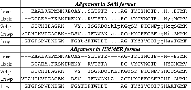 |
To be able to compare the model building and scoring of the two packages
independently it is necessary to convert between the SAM and HMMER
model formats, and so a program
(http://www.mrc-lmb.cam.ac.uk/genomes/julian/convert/convert.html)
was written by Martin Madera for this purpose. The program can convert
between the HMMER and SAM model formats with the minimum loss of information.
There is a difference in the architectures of the models which means
that there is some unavoidable information loss when converting from
a SAM model to a HMMER one, but none is lost the other way. See the
web site for further information (written by Martin Madera).
The SUPERFAMILY sequence set filtered to 40% sequence identity was used in the SCOP test (see chapter 2). There are 2892 sequences in this set, with approximately 40000 possible true pair-wise hits at the superfamily level. Models generated from every sequence were scored against all sequences for each method. This all against all comparison allows a very diverse and un-biased (between methods) comparison on a large amount of data.
To compare the SAM and HMMER programs, models were built from independent multiple sequence alignments. The multiple sequence alignments were generated from a single seed sequence in each case in two possible ways:
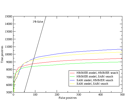
|
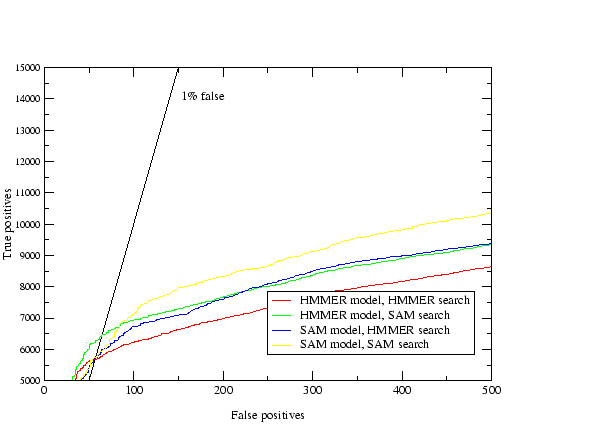
|
Work done by Martin Madera on a wide range of alignments for the Cupredoxin and Globin families showed that SAM model building and SAM scoring was better than HMMER model building and scoring. This conclusion seems to be partially in agreement with the results in graph 5.1 and fully in agreement with the results in graph 5.2. In all cases SAM model building performs better than HMMER model building, and in 5.2 SAM scoring performs better than HMMER scoring, but in 5.1 HMMER scoring performs better than SAM scoring. One possible explanation (which turns out not to be true) is that the HMMER E-values are more consistent than the SAM E-values as a consequence of model calibration. If this were true SAM would have a better true-false positive rate in individual cases where only the separation of true from false homologues counts. In the case where all of SCOP is used, the true-false positive rate is for all searches at a fixed E-value, so the consistency of the score is just as important as the ability to separate true from false homologues. However, plotting the number of true hits before the first (or 2nd or 3rd) false hits for each model, rather than the number of true and false hits before a given E-value, yields the same behaviour as before (figure 5.3 corresponds to figure 5.1).
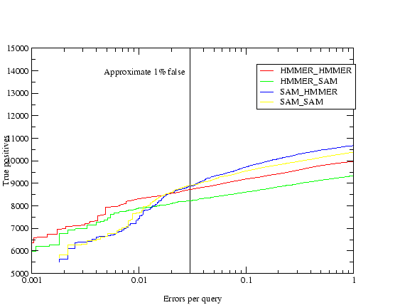
|
In the case of the globins and cupredoxins, the alignments used for model-building were all high quality diverse alignments without large insertions. In the case of the alignments used in the SCOP BLAST tests, rather than the work by Martin Madera and the SCOP T99 tests, the alignments were less diverse lower quality alignments with large insertions due to ClustalW. SAM builds the model architecture based on the information about deletions and insertions in the alignment, whereas HMMER is able to `decide' for itself. As a consequence the SAM models have one segment for every column in the alignment, whereas HMMER consigns some columns to be insertions. As a result HMMER builds better models from poor alignments than SAM, but SAM builds better models from good alignments than HMMER.
The result that HMMER performs better than SAM with poor alignments and vice versa, suggests that the match regions specified in the alignments (by upper case letters) are superior to the match regions chosen by HMMER for the good alignments, and worse for the bad alignments. If this is true, it should be possible to improve the performance of HMMER with the good quality alignments by not letting HMMER `decide' the match states. It is possible to specify the match states by hand in the HMMER model building procedure.
A program (http://stash.mrc-lmb.cam.ac.uk/SUPERFAMILY/a2m2selex.html)
was written to convert alignment information into match and insert
state information which can be passed to HMMER using the `-hand'
option in combination with the `selex' format. In this way the information
in the alignments is used implicitly, but this cannot be regarded
as default operation of the HMMER procedure. This was done for the
best-performing procedure which uses the T99 script to generate alignments
with full upper and lower case characters specifying the aligned and
unaligned regions (see figure 5.4). The results suggest that
there is very little difference between SAM and HMMER when using the
alignment information to specify the states of the model, with SAM
doing marginally better. A little performance is lost in converting
between the formats.
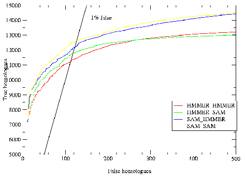
|
The null scoring in SAM and HMMER is quite different [63], as HMMER uses its `null2' model and SAM uses the `reverse-null'. The effects of the null scoring are mostly covered by the SCOP tests, but the low complexity and repeat masking aspect is not (due to the lack of such sequences in the PDB).
A short test was made of the ability of both methods in this respect; WU-Blast was also included in the test. 100 models from different SCOP folds were chosen as a test set, and they were scored against three databases of sequences with roughly 2000 sequences in each:
The speed of the programs is important because this may determine the feasibility of large scale experiments. Although all of these methods perform much better than Blast at remote homology detection, Blast is so much faster that it can be used on a scale these methods cannot. The time taken for the model-building , model-calibrating, and model-scoring was recorded for 100 cases, and the average times compared. The cases vary in length, complexity and abundance of homologues. The models were all scored against 1159 sequences (see figure 5.5).
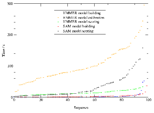
|
The model-building is very quick using both methods and so is not very important, however it is worth noting that HMMER model calibration is very slow and, if this is included in the time required to build a model then HMMER is many orders of magnitude slower. The model-scoring was approximately twice as fast when using HMMER, but a difference of this size means that there are not many uses for which SAM would not be appropriate and HMMER would be. This extra time results from SAM calculating the score for both the actual sequence and its reverse, doubling the time taken. This is largely for the purpose of eliminating hits to low complexity sequence and repeat regions. Model calibration in HMMER scores 5000 sequences by default during the process, which is the cause of the cost in time. If a single model is to be built and then scored once against 5000 sequences, it is roughly estimated that SAM and HMMER will take the same time. This is because HMMER effectively has to score 5000 sequences in calibration and then 5000 in the search, whereas SAM only scores 5000 sequences (but in both forward and reverse directions), resulting in the same time. If over 5000 sequences are to be scored, then HMMER is on average roughly between 1 and 2 times as fast as SAM.
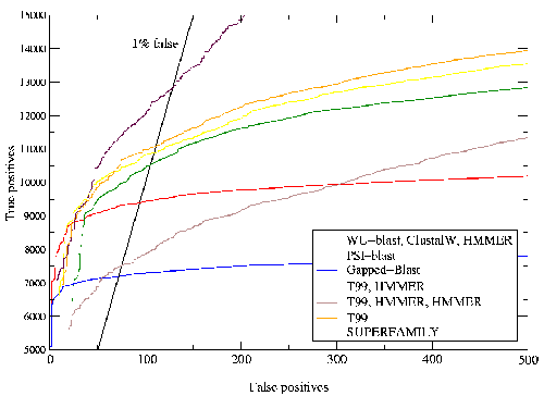
|
In order to see the performance of SAM and HMMER in the context of other sequence comparison methods, other all against all comparisons were made (see figure 5.6):
It is clear from the results that the most significant distinction between the SAM and HMMER packages as a whole is the SAM T99 script. Not only do both packages require a multiple sequence alignment from which to build a model, but their performance is directly related to the quality of that alignment. The SAM-T99 script produces high quality multiple alignments well suited for building HMMs, yet there is no equivalent in the HMMER package. Bearing this in mind, the other individual components of the packages may be compared separately, namely model building from an alignment and model scoring from a model.
The greatest difference between the two methods in model building is the way in which the alignment information is used. The SAM model architecture is taken directly from the alignment, and this information must be specified using upper and lower case characters. The HMMER model architecture is deduced from the residue frequencies of columns in the alignment alone, ignoring the case. As a consequence if the alignment is poor, or more specifically if the definition of the aligned and unaligned regions (upper and lower case) is poor, then HMMER will build better models, whilst SAM inherits an inappropriate architecture from the alignment. On the other hand if the alignment quality is good, with well-specified regions of aligned and unaligned (upper and lower case) columns, SAM will inherit the benefits whereas HMMER will not. In these cases the SAM models will be superior due to the architecture specified in the alignment.
It should be noted that the architecture generated in the alignments from the SAM T99 script, is superior to that which HMMER creates from the same alignment. It is possible to extract the architecture from the alignment and specify it by hand for the HMMER model, forcing it to have the same architecture as the SAM model. In this case there is little difference between the methods, but this is not the default procedure. Likewise there are programs in the SAM package for automatically improving the architecture as HMMER does, but these are not considered here as they also are not part of the default SAM procedure either. It is thus the default method of specifying the model architecture which separates SAM from HMMER, not the underlying algorithm.
It is possible using Martin Madera's script to convert between the SAM and HMMER model formats, and so score the models with either package. Both SAM and HMMER programs appear to work better in conjunction with their own packages, which is observed by a small general loss in performance when models are built and scored using different packages. These differences are greater when poor performance is being achieved. This result is apparent from work by Martin Madera on the Globin and Cupredoxin families.
The E-value scores produced by both methods have similar reliability, but to achieve this HMMER models must be calibrated which is an equivalent computational cost to scoring 5000 sequences. The greatest difference between the two methods in model scoring is due to the treatment of low complexity and repeat sequence filtering, which is effective in both. HMMER achieves this with the HMMER `null2' model and SAM uses the different approach of off-setting the score against the score of the same sequence in reverse. This means that HMMER scoring is approximately twice as fast as SAM scoring. If model calibration is included then SAM scoring is faster for searches of less than 5000 sequences and HMMER is faster for scoring more than 5000 sequences.
This chapter aims to compare the SAM and HMMER hidden Markov model software packages. Because the method's performance is dependent on the expertise of the user, the aim is to carry out all comparisons using the default procedures, as an inexpert user would.
The evidence suggests that there is little difference in the overall performance of SAM and HMMER, yet SAM does on average perform slightly better. In conclusion both SAM and HMMER are excellent packages for remote homology detection, with small differences in the performance of the individual algorithms. The undeniable advantage however lies with SAM due to the T99 procedure which is essential for automatically producing high quality models.
The work also confirms that profile methods perform very much better than pair-wise methods, and that HMMs perform better than PSI-Blast.
This thesis describes the development of the model library, but the more general direction is to use this model library to carry out structural domain assignments to the sequences of complete genomes. This chapter describes the application of the model library to large scale genome studies.
The computational problem of scoring all models against all sequences in a genome is merely a technical one, but there are also two conceptual problems. Firstly as explained in previous chapters a superfamily is represented by a group of models rather than a single model. As a consequence any given sequence may have significant hits to more than one model in the superfamily. Secondly, it is possible that a sequence hits more than one superfamily as an inevitable scoring error. The difficulty is not in deciding which assignment is more significant (given by the score), but in deciding whether or not two hits are in conflict with each other. For example if there are two overlapping assignments, a decision must be made as to whether they are in conflict and one is false, or whether the predicted domain boundaries are incorrect and both are correctly assigned. This problem is particularly obvious for inserted domains where the boundaries of one domain lie completely within another.
Sarah Teichmann had previously carried out structural assignments to the Mycoplasma genitalium genome [65] using PSI-Blast. The problem of conflicting assignments is the same here. The way in which the assignments were dealt with in this work was that the beginning and end of any two assignments to the same sequence were compared. Any two regions overlapping by more than a fixed number of residues were considered to be in conflict and the one with the highest score was kept.
Initially some improvements were made to the above procedure previously employed by Sarah Teichmann, but these attempts to improve things ultimately lead to a completely different approach (following sub-section).
The first improvement was that the overlap was expressed in terms of the fraction of the shorter sequence involved in the overlap. This is because the linker regions of some large proteins (example of areas of expected inaccurate location of domain boundaries) may be similar in length to entire small proteins. Due to this an absolute number of residues in an overlap is not appropriate.
To account for inserted domains the expected length of a domain was taken into account. The length of the model was subtracted from the length of the hit, so that an estimate on the amount of inserted sequence is made. This number is subtracted from an overlap used to decide the conflict. In this way inserted domains are allowed, and some large insertions due to mis-alignment (usually at the edge of a domain) do not produce a conflict where there should be none.
The procedure by which the scores of the hits are compared is essential for obtaining an optimal set of matches. A conflict between two hits causes the one with the less significant score to be rejected, but the order in which the comparisons are made affects the final result. The hits are ordered on score, and the most significant one is always kept. The other hits are then compared in order until another one is kept. The comparisons then continue down the order but are compared to all hits which have so far been kept. This gives the best possible combination of non-conflicting domain assignments. For example if a hit of very low significance conflicts with one of medium significance, it is kept if the hit of medium significance is in conflict with one of very high significance.
When using the model library, there is the additional problem of comparing the multiple hits to the same superfamily. This is solved in the same manner as inter-superfamily conflicts but with much more restrictive parameters.
This assignment procedure was applied to 22 genomes and the effect of the percentage overlap examined. The same percentage was used for inter and intra-superfamily assignment. Figure 6.1 shows that as the required overlap increases so does the number of assignments. This is obvious from the assignment procedure, but what the graph also shows is that it is roughly logarithmic between 5 and 75 percent overlap. Outside this region the steeper increase in assignments suggests that only a threshold for conflict within the region would be reasonable.
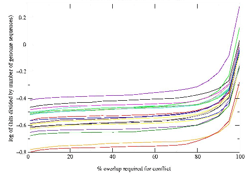
|
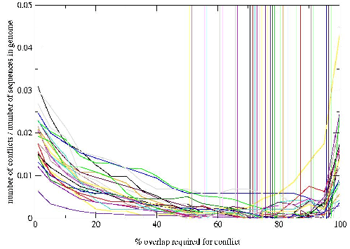
|
To improve the assignment procedure still further an analysis of the expected lengths of domains was carried out. The mean and standard deviation of lengths in each superfamily were calculated and incorporated into the assignment procedure.
At this point the visual inspection of the alignments in many cases lead to the decision that the way forward was not to continue developing the procedure with ever-increasing complexity. The alignments themselves were used in a new procedure.
The final procedure which was developed and is used in the work in the following sections compares the alignments of every hit. Given any two hits to a sequence, the sequence is aligned to the models in question. Every residue in the sequence which passes through a match state in both models is considered to be in conflict. Summing all of the conflicting residues gives the overlap. This number is consistently much smaller than the overlap obtained with the previous method, and distinguishes well between overlapping regions of strong conflict (well-aligned) and weak conflict (sparse and badly aligned). This method has only two variable parameters: the percentage overlap required for conflict, and the minimum core size. A range of values was explored for these parameters but unlike the previous method the results were robust and not very sensitive to variations. A conservative overlap of 20% was chosen to define a conflict and the minimum core size was set at 30 residues. Any overlap causing an assignment to have less than 30 residues after subtracting the overlap is taken as a conflict.
This procedure using the alignments simultaneously solves the problem of inserted domains and overlapping assignments, both for inter and intra-superfamily selection of hits. Work by Sarah Teichmann analysing in detail the non-contiguous assignments, examining inserted domains, long sequence matches and overlapping assignments made to genomes sequences found only four errors in 3041 assignments.
The model library in conjunction with the assignment procedure and some scripting software forms a complete package for structural domain assignments. This has been applied to 56 complete genomes, and some other sequences.
The genome assignments were carried out on the peptide sequences resulting from the gene predictions carried out by each genome project. The majority of these were downloaded in FASTA[20] format from the National Centre for Biotechnology Information (NCBI http://www.ncbi.nlm.nih.gov). Some particular genomes were downloaded from the official site for the genome project, for example the human genome at ENSEMBL (http://www.ensembl.org), and some via personal communication (e.g. Arabidopsis thaliana).
A model library based on the 1.53 release of SCOP was used to carry out structural superfamily assignments of 56 complete genomes. The domains within sequences which hit with a significant score were uniquely assigned to a superfamily. The assignments cover roughly 45% of prokaryotic and 35% of eukaryotic genome peptide sequence.
No significant difference in the distribution of the scores given to each assignment was found between genomes. Differences were found however between the distributions for each genome of the sequence identities between the matched genome sequences and the sequences used to seed the HMMs (figure 6.3).
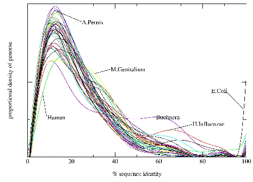
|
As well as giving assignments that can be used in new investigations into genomes, they provide potential new annotations. An analysis of sequences previously unassigned showed that in most genomes the SUPERFAMILY HMMs detect large numbers of novel assignments. The extent of this varies greatly with the quality of annotation carried out on the genomes by the sequencing projects (figure 6.4).
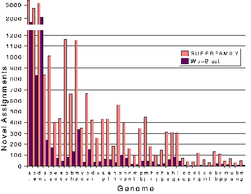
|
The coverage of the genomes is shown in figure 6.5.
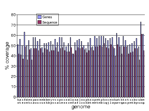
|
Each genome the tables 6.1 and 6.2 show in order:
the name of the species of the genome(genome); a 2-letter code (A);
the domain where `E' is for eukaryota, `A' is for archea and `B' is
for bacteria (B);the number of genes comprising the genome(C); the
number of genes which have at least one SCOP domain assigned(D); the
percentage of genes with at least one domain assigned(E); the percentage
of the actual sequence covered by SCOP domains because multi-domain
genes may have some domains assigned but not others(F); the total
number of domains assigned(G); the total number (out of a possible
859) of superfamilies represented by at least one domain in the genome(H).
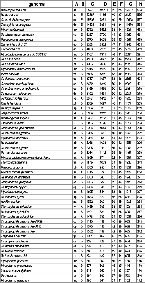 |
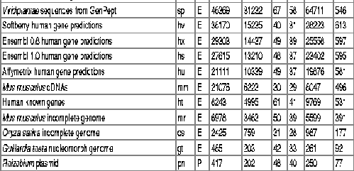 |
The extensive set of genome assignments is best represented in these summary tables, but the detail of the stored data is much greater. The data is too large for an appendix, so the reader is referred to the database described in the following chapter. The structural annotation of the genomes presented in this work makes it possible to make evolutionary inferences not previously possible. Collaborative work [8,9] has already been carried out using this data and more is in progress.
Comparing all of the assignments to eukaryotes (see figure 6.6 ) shows that most domains are common to all eukaryotes, and that most of the domains in eukaryotes belong to the same superfamilies. This implies that almost all of the evolution leading to new genes in eukaryotes since an ancient common ancestor has occurred by gene duplication and recombination, followed by subsequent mutation and divergence.
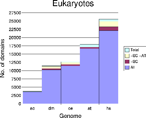
|
Comparing all of the assignments to bacteria in figure 6.7 shows that most domains are common to two of the larger genomes (Escherichia coli and Bascillus subtilis), and that most of the domains in bacteria thus belong to the same superfamilies. This implies that almost all of the evolution leading to new genes in bacteria since an ancient common ancestor has occurred by gene duplication and recombination.
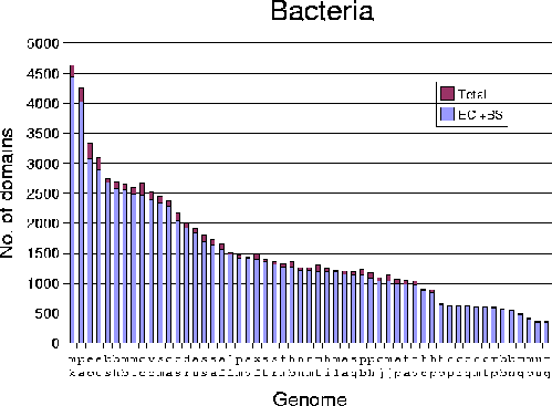
|
To give a feel for how the assignments can be used for genome analysis from the point of view of an organism, one is singled out and compared to the others. Arabidopsis thaliana is a small flowering plant whose complete genome is compared to the others here. It is a very large genome, second at the moment only to human (incomplete). Mycoplasma genitalium has the smallest known genome yet still contains 15 superfamilies arabidopsis does not have. The human genome contains 110 not present in arabidopsis, whereas arabidopsis contains 75 which human does not.
P-loop hydrolases are the most abundant superfamily in every genome apart from Drosophila melanogaster (whose top superfamily is the zinc finger) and human (zinc finger, immunoglobulin, EGF/Laminin). The protein kinase superfamily is the second largest superfamily in arabidopsis which is very large in all eukaryotes, and very small in prokaryotes .Rossmann domains, tetratricopeptide repeats (TPR), homeodomains, and alpha/beta-hydrolases are all in the top ten arabidopsis superfamilies, and are also abundant in most other genomes. Also in the top ten are RNI-like, RING, RNA-binding, and ARM repeat domains which are common in all eukaryotes, and not usually present in prokaryotes. RNI-like, RING, and tetratricopeptide repeat (TPR) domains are all 2-3 times more common in arabidopsis than any other genome. There are no cadherins, spectrin, SCR, Fibronectin III, or lectins which are common in other multi-cellular organisms. There are however ten plant lectin domains (of which there are also seven in the Caenorhabditis elegans genome).
The genome was examined for unique or over-represented superfamilies, and the following points were worthy of note.
So far the model library has been applied only to amino acid sequences. In the case of the genomes they rely on the gene predictions carried out by the genome projects. It is possible to search nucleotide sequences with no prior gene prediction.
To carry out the search the nucleotide is simply translated into amino acid sequence and scored against the models that way. There are six frames which the nucleotide must be split into, three on each strand of the DNA. The nucleotide sequence is translated into the six reading frames and split into separate sequences at every stop codon. Fragments shorter than 10 residues are disregarded as they will not be assigned a significant score.
Although the results of a DNA search carried out in this way will be incomplete and potentially contain pseudo-genes, it is still a valuable analysis and can be used as an aid to automated gene prediction.
Assignments were carried out to six human genome contigs (contiguous lengths of nucleotide sequence) approximately 200,000 base pairs in length. Figure 6.8 shows the assignments to the raw nucleotide sequence.
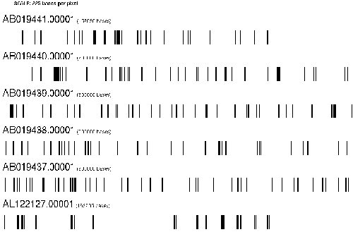
|
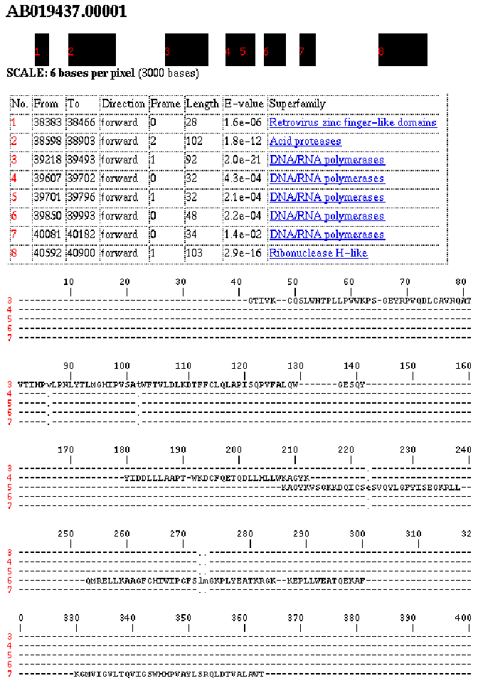
|
The Guillardia theta nucleomorph genome is the most gene rich eukaryote sequence known at the time of writing, and is sufficiently small to carry out a complete analysis on. The analysis has been carried out and the data is available in an interactive manner using hypertext pages in the manner of the graphs for the human contigs. As this data is unsuitable for an appendix the reader is referred to http://stash.mrc-lmb.cam.ac.uk/SUPERFAMILY/guillardia.
This chapter describes the development and implementation of an assignment procedure for use with the model library described in previous chapters. The assignment procedure in conjunction with the model library has been used to carry out structural assignments on all completely sequenced genomes at the time of writing.
The result is that a very large quantity of data has been generated and organised which is expected to become the starting point of other projects. The technical issues have not been discussed here but much of the work involved in creating what is presented here was computationally demanding.
The model library is the means to the end of this thesis, which is the genome assignments.
The model library and genome assignments, and some associated software have been used to create the SUPERFAMILY database. The database is available on the world wide web at http://stash.mrc-lmb.cam.ac.uk.
All of the data is all held in an SQL relational database [67]. Perl CGI scripts are used to query the database and generate server side dynamic html pages, served by an Apache web server [68] on a machine running Linux [69]. The server is a dual-processor 500Mhz with 1Gb of RAM which was assembled from separate parts. The server also serves the PDB-ISL[58] database. Figure 7.3 shows a screen shot of the front page of the server.
The server processed over 1,500 sequence requests last month (august), which is an increase of a factor of ten from the beginning of the year (2001). In the same month there were visits to the web site from over 1,500 different sites, accessing nearly 20,000 pages.
The following services are provided by the server.
The most obvious service to provide is the ability to search the model library. Users may submit up to ten amino acid or nucleotide sequences to the server at any time. Notification of completion of the result can be returned by e-mail or via the browser; upon completion web pages are created for viewing the results. A single query takes approximately five minutes, but can take longer if the query is particularly long. The results are displayed as in figure 7.2. The E-value associated with each domain assignment is given, as well as the region of the query sequence which it covers. The superfamily has a link to the SCOP web site, and there are buttons linking to the alignment and genome assignments (see later).
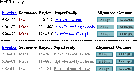
|
Another service provided by the server is multiple alignments to the models in the library. Both the actual alignments and sequence searches rely on the underlying SAM software. Built into the server are all of the PDB sequences, all of the genome sequences, and all of the sequences in the alignments from which the models were built. Any number of these sequences can be selected aligned to a model as described in a previous chapter. See figure 7.3 for an example alignment from the server.
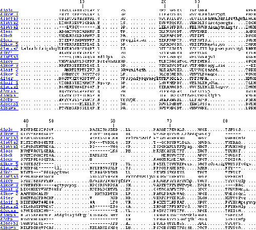
|
The link from the search results page takes the user to an alignment of the query sequence to the assigned domain. It is also possible for the user to enter their own sequences, or upload a sequence file from their local computer. There are links to alignments of genome sequences from the genome pages described next.
From each alignment page there is a link to a statistical breakdown of the multiple alignment. This is very useful in combination with structural analysis for identifying the functional determinants [34]. This breakdown gives data on every column of the alignment: the occurrence of every residue, occurrences of the hydrophobic/hydrophilic/neutral groups, the log odds probability of the key features, and also the mean and standard deviation of the volumes of the residues. In the appendix there is an example of these statistics generated on the cupredoxin alignment in the first chapter.
All of the genome assignments are available from the server. The main genome page contains a table similar to tables 6.1 and 6.2, with a link to a separate page for each genome, for example figure 7.4. At the top of the page are links to the source of the genome, the taxonomy and some summary information. Following that is a list of all superfamilies in order of size (number of domains assigned). Each superfamily links to another page with a complete listing of all domains in the genome assigned to that superfamily. It is also possible to view and compare on the same page all of the assignments to that superfamily in other genomes. Finally for each domain assignment there is a cross-reference to the whole gene on another page the same in appearance as the results page from a sequence search (figure 7.2). All of these pages have links to alignments of the sequences.
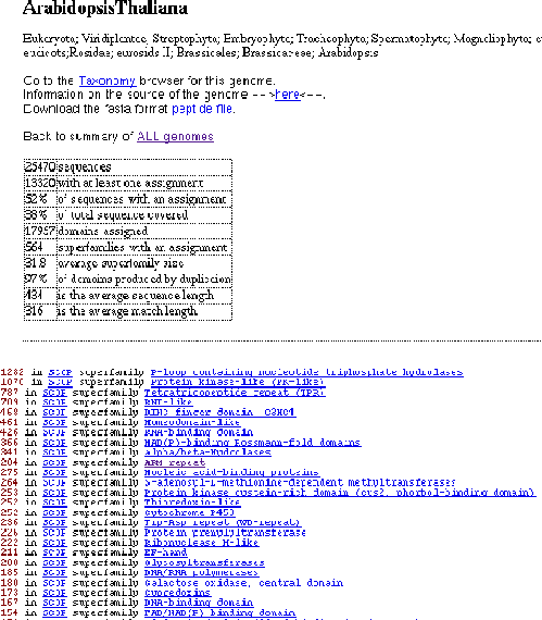
|
The SUPERFAMILY database also runs a distributed annotation system (DAS) server running for the human and worm genomes. DAS (http://www.biodas.org) is a protocol for a de-centralised annotation of genomes [70]. The user has a client which they can use to view the genome, and then choose the annotation tracks which they wish to view in the genome. Each annotation track can be served by a different DAS server, with the client contacting all chosen servers and retrieving their annotation to be viewed alongside each other in the same browser (the client). The SUPERFAMILY server supplies the SCOP structural domain assignments as a possible track on the genome. A reference server is required by the client for each genome, and there are only a few reference servers available at the time of writing, so only annotations to human and worm (fly genome is in progress) are currently served. There are not yet very many servers available for use with DAS yet and the system is still under development, however it is important to look to the future and such a standard protocol is essential for bringing together resources.
The superfamily DAS annotations are available from http://stash.mrc-lmb.cam.ac.uk:8080/das and are served by a Tomcat server running a Java virtual machine. The DAS servlet is part of the biojava project, and the datasource plugin was written by Thomas Down. The servlet uses the datasource plugin to query the underlying SQL database (mentioned earlier) for the assignments.
The SUPERFAMILY server can respond to automatic server requests from computers as well as individual users. There are two external meta servers which regularly make use of this function: the `META PredictProtein' server at http://cubic.bioc.columbia.edu/pp/submit_meta.html, and the `Meta-Server' server at http://bioinfo.pl/meta. Both of these sites link together a collection of resources, enabling a user to do a single submission which gets sent to all of the servers (of which SUPERFAMILY is one), and in the case of `Meta-Server', the progress is monitored and the results parsed into a common format [71].
Given an assignment of a sequence to a known structural domain it is possible with an accompanying alignment to generate a three-dimensional model using the known structure as a template. Figure 7.5 shows a three-dimensional structural model using a beta propeller as a template. This paraoxonase (PON1 [72]) sequence was a very distant homologue to a known structure (1e1a) at the time of the prediction (SCOP 1.53), and had a function previously unobserved in beta propellers. Since then a new beta propeller structure has been solved with a much higher similarity to the PON1 sequence. This new structure had the same function so the prediction turned out to be accurate in this case.
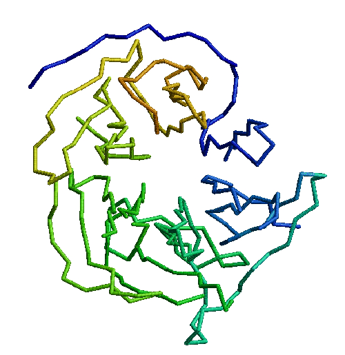
|
The server can automatically supply 3-D models which are required by the automatic assessment methods described in the next section.
The model library performs extremely well in validation tests against SCOP but, as it has been heavily trained on these validation tests themselves, the rigorous test is one of blind prediction such as the CASP[62] test. SUPERFAMILY was submitted to LiveBench (http://bioinfo.pl/LiveBench) which continuously benchmarks prediction servers, which is based on the CASP concept and offers difficult targets of recently solved structures. All targets have a BLAST[21] E-Value higher than 0.1 to all other members of PDB. Out of the 203 targets in the LiveBench-2 project (collected between 13.4.00 and 29.12.00), 45 were assigned to the correct SCOP superfamily by SUPERFAMILY and one falsely assigned. The one incorrect assignment involved a very short cysteine-rich protein and sequences of this kind are known to produce false matches with good scores[32].
The server was submitted to the EVA project (http://maple.bioc.columbia.edu/eva) over six months ago, and a great deal of requests from the EVA project have been processed. Unfortunately there are no results available on the web site yet.
To assess the improvement in the detection of homology made by the SUPERFAMILY HMMs described here, their performance was compared with that of a pairwise sequence comparison method. For this comparison we used WU-BLAST because previous work has shown that this is one of the most effective of the pairwise methods[32]. The 4849 SCOP 1.53 sequences that were used to seed the SUPERFAMILY HMM models were directly matched by WU-BLAST to the sequences of the complete genomes. For this calculation WU-BLAST version 2.0a19 was used with default parameters and matrix (BLOSSUM62). All those WU-BLAST matches with P values of less than 0.001 were taken as significant. This P value is expected to select matches whose significance is the same as the SUPERFAMILY scores[48].
The ratio of the number of sequences matched by the two methods is very similar for the different genomes: the WU-BLAST procedure makes matches to half the number of sequences that are matched by SUPERFAMILY. On a more detailed level we compared the number of "hypothetical" sequences matched by the WU-BLAST and SUPERFAMILY procedures. At this level WU-BLAST matched between 4% and 36% of those matched by the SAM HMMs (see figure 6.4).
The coverage presented in table 6.1 shows that 54% of the genes of Mycoplasma genitalium have a structural assignment. The current SUPERFAMILY HMM library which has been recently updated to release 1.55 of SCOP has structural assignments to 61% of the genes. It is possible to compare coverage for this genome with many other methods because it is very small (480 sequences) and so most methods have a comparable analysis. GenThreader[73] covers 53% (Jones, personal communication) of the genes, but is computationally costly and as a consequence has not been applied to many genomes. PSI-BLAST[28] has been used by several groups yielding coverages of 37% (Huynen et al. [74]), 39% (Wolf et al. [75]), and 41% (Teichmann et al. [65]). These figures were obtained using the fewer PDB sequences available at the time. Much more extensive use has been made recently by Gene3D (http://www.biochem.ucl.ac.uk/bsm/cath_new/Gene3D) which covers 41% of Mycoplasma genitalium proteins, and has been applied to over 30 genomes including 2 of the smaller eukaryotes. Gene3D is based on the CATH [76] database. None of these methods have been applied as extensively as the work presented here however, and most notably there is a lack of analysis of larger eukaryote genomes. A detailed comparison to 3 other methods is shown in section 7.2.3.
As mentioned above the most extensive structural assignments to genomes other than the work presented here is by the Gene3D project at University College London by Daniel Buchan, Dr. Frances M.G. Pearl, Dr. Adrian J. Shepherd, Dr. David Lee, Dr. Christine A. Orengo, Prof. J.M. Thornton, Stuart Rison and Ian Sillitoe. This database is the most similar to SUPERFAMILY and the coverage of the genomes from each of the databases are compared in figures 7.6 and 7.7. This comparison was made some months ago in February 2001. All of the genomes from both databases are included, some of which were not included in one or the other at the time. SUPERFAMILY now contains all 56 complete genomes whilst GENE3D only covers those shown here, most notably only two eukaryotes: yeast and worm. Some of the assignments made by GENE3D are so poor (e.g. `cp') that there must be some error, which has not been fixed at the time of writing.
|
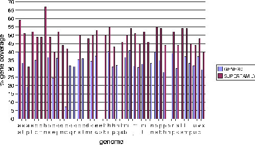
|
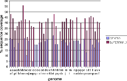
|
To examine the nature of the overlap between the assignments made by SUPERFAMILY and by other state of the art methods, the differences in the assignments between SUPERFAMILY and three other methods were compared. The three methods were Gene3D, GenThreader, and the structural families in PFAM. All data for this comparison were provided by the authors of the methods at the same time (March 2002). These were partly chosen because of the availability of their data, but also because they are representative of the available structural assignments to genomes. Gene3D uses the CATH database, which is the main structural classification other than SCOP, and PSI-BLAST which is the main iterative profile method other than SAM-T99. GenThreader is the most conceptually different procedure, and the only one with a coverage of the genome similar to SUPERFAMILY. PFAM is a HMMER-based database and has been as widely applied to genomes as SUPERFAMILY, so is a good comparison with respect to the improvements in the HMM procedures discussed here.
There are 168 sequences out of a possible 480 which have assignments made to them by all four methods, and each method individually makes assignments to between 196 and 303 sequences. Figure 7.8 shows the overlap of the sequences which have assignments from the four methods, the details of which are discussed in detail below.
The assignments made by SUPERFAMILY which are not made by other methods are examined to determine whether they are true or false, and to discover in which areas they occur. SUPERFAMILY assignments were made to 107 sequences with no assignment by Gene3D, 96 with no assignment by PFAM (families with a structural representative), and 46 with no assignment by GenThreader. In SUPERFAMILY 50 assignments were made to the 46 sequences with no GenThreader assignment. These were examined in detail:
The distribution of assignments found by SUPERFAMILY and not found by GenThreader did not follow any pattern. No single model was responsible for more than one of the additional hits, with the exception of one model which was responsible for two. This suggests that there is no systematic error or advantage in any particular model. The only assignments which could be grouped were five ribosomal proteins, which were all assigned by different models and all annotated as ribosomal proteins by the genome project.
Although the distribution of assignments found by SUPERFAMILY but not by PFAM or Gene3D were not verified as true or false due to the magnitude of the task, it is still interesting to compare the differences. Of the 107 sequences without assignments by Gene3D, 39 had PFAM assignments to known structures, and of the 96 without assignments by PFAM, 26 had Gene3D assignments.
The distribution across the SCOP classification of all assignments made by SUPERFAMILY but missed by one of the other methods is surprisingly even and shows no particular area in which SUPERFAMILY is succeeding more than the other methods. The 50 assignments to sequences with no assignment by GenThreader span 37 SCOP superfamilies (see table 7.1), the 96 sequences with no PFAM assignment span 63 superfamilies, and the 107 sequences with no Gene3D span 80 superfamilies. The distribution across SCOP classes shows relatively more assignments to the larger classes such as `alpha and beta proteins (a/b)', and fewer to smaller ones such as `Multi-domain proteins (alpha and beta)'. There are also more hits to the families which are more highly represented in the Mycoplasma genitalium genome, most notably the P-loops. This distribution would be expected if there were no particular bias towards certain areas.
| True/False | SCOP | ID | Superfamily description |
| T | a.2.2 | MG159 | Ribosomal protein L29 (L29p) |
| T | a.4.5 | MG101 | "Winged helix" DNA-binding domain |
| T | a.4.5 | MG205 | "Winged helix" DNA-binding domain |
| T | a.60.2 | MG206 | RuvA domain 2-like |
| - | a.87.1 | MG103 | DBL homology domain |
| - | a.93.1 | MG099 | Heme-dependent peroxidases |
| T | b.34.5 | MG162 | Translation proteins SH3-like domain |
| T | b.40.4 | MG376 | Nucleic acid-binding proteins |
| T | b.43.3 | MG151 | Translation proteins |
| T | b.47.1 | MG067 | Trypsin-like serine proteases |
| T | b.47.1 | MG068 | Trypsin-like serine proteases |
| - | b.50.1 | MG369 | Acid proteases |
| T | b.55.1 | MG067 | PH domain-like |
| T | b.60.1 | MG185 | Lipocalins |
| - | b.82.3 | MG352 | cAMP-binding domain-like |
| - | b.86.1 | MG101 | Hedgehog/intein (Hint) domain |
| T | c.1.9 | MG009 | Metallo-dependent hydrolases |
| - | c.1.16 | MG184 | Bacterial luciferase-like |
| T | c.12.1 | MG169 | Ribosomal proteins L15p and L18e |
| T | c.21.1 | MG418 | Ribosomal protein L13 |
| T | c.26.1 | MG240 | Nucleotidylyl transferase |
| T | c.37.1 | MG110 | P-loop containing nucleotide triphosphate hydrolases |
| T | c.37.1 | MG315 | P-loop containing nucleotide triphosphate hydrolases |
| T | c.37.1 | MG442 | P-loop containing nucleotide triphosphate hydrolases |
| - | c.37.1 | MG442 | P-loop containing nucleotide triphosphate hydrolases |
| - | c.47.1 | MG312 | Thioredoxin-like |
| - | c.47.1 | MG127 | Thioredoxin-like |
| T | c.52.1 | MG373 | Restriction endonuclease-like |
| T | c.55.1 | MG046 | Actin-like ATPase domain |
| T | c.66.1 | MG222 | S-adenosyl-L-methionine-dependent methyltransferases |
| - | c.69.1 | MG281 | alpha/beta-Hydrolases |
| - | c.79.1 | MG100 | Tryptophan synthase beta subunit-like PLP-dependent enzymes |
| T | c.91.1 | MG085 | PEP carboxykinase-like |
| T | c.94.1 | MG260 | Periplasmic binding protein-like II |
| T | c.94.1 | MG321 | Periplasmic binding protein-like II |
| T | d.41.4 | MG158 | Ribosomal protein L10e |
| T | d.64.1 | MG100 | eIF1-like |
| T | d.66.1 | MG209 | Alpha-L RNA-binding motif |
| T | d.66.1 | MG370 | Alpha-L RNA-binding motif |
| T | d.144.1 | MG356 | Protein kinase-like (PK-like) |
(Continued overleaf) A table showing the 50 assignments made by SUPERFAMILY to sequences with no assignment by GenThreader.
|
The assignments made by other methods to sequences for which SUPERFAMILY has no assignment are examined to determine whether they are true or false, and to determine what SUPERFAMILY is missing which should be detectable from the sequence. Of the sequences with no SUPERFAMILY assignment, there were none with an assignment by Gene3d, two with an assignment by PFAM (structural families), and 78 assignments to 35 sequences by GenThreader. The two PFAM assignments were both confirmed as true by the genome annotation. The 78 assignments by GenThreader were examined in more detail.
The hits found by GenThreader and not by SUPERFAMILY were often to the same sequences, and sometimes to the same structural template. This is suggestive of a problem causing repeating errors. Further to this most of the assignments were involved with coiled coils, repeats, and alpha superhelices. It was found that 26 out of the 35 additional sequences found by GenThreader were annotated by the genome project as `conserved hypothetical protein' or `predicted coding region', whereas only 15 out of 50 of those found in addition by SUPERFAMILY were.
|
The Mycoplasma genitalium genome is probably not representative of all genome assignments, especially those in higher eukaryotes, but this comparison gives some indication of the differences between SUPERFAMILY assignments and the other state of the art methods. SUPERFAMILY makes assignments to many more sequences than Gene3D or PFAM structural families, but approximately the same number as GenThreader. Largely the PFAM and Gene3D assignments are redundant to the SUPERFAMILY ones. GenThreader makes assignments to a similar number of sequences, but there are appreciable differences between them and the SUPERFAMILY assignments. Most of the assignments made by SUPERFAMILY and not made by GenThreader can be shown to be probably true, and few can be shown to be probably false. This indicates that the additional genome coverage obtained by SUPERFAMILY is likely to be genuine. Many of the assignments made by GenThreader and not by SUPERFAMILY can be shown to be false, and a much smaller proportion can be shown to be true. This, in conjunction with the almost complete redundancy of the PFAM and Gene3D assignments, indicates that SUPERFAMILY is not missing many assignments which other methods are able to find reliably.
Finally examination of the extra coverage found by SUPERFAMILY indicates that the improvement is across the board, with no particular emphasis on any SCOP class or superfamily, or from any particular SUPERFAMILY models.
The work presented in this thesis has many applications for other work. Some of uses which it has already been put to are listed in this section.
The WWW server described in this chapter has been used on many projects for sequence searches, alignments, and genome assignments as mentioned above. It has been used for teaching in several universities.
Some other servers rely upon the work shown here.
The Human Immunoglobulin Hits database (HIGH) at http://www.genomesapiens.org uses the IG assignments to the human genome by SUPERFAMILY from several releases of ENSEMBL (see next). Additional work is done by Bernard Debono on the assignments to verify, improve and extend them for presentation in the HIGH database.
The ENSEMBL database at http://www.ensembl.org provides the human genome data from the public sequencing project [84]. The ENSEMBL pipeline for annotation uses the SUPERFAMILY models and assignment procedure to annotate the peptide sequences from the gene predictions with SCOP structural domains. The assignments appear on their web-site as part of their annotation alongside other annotations such as PFAM[51].
Ewan Birney of the ENSEMBL project is currently working on incorporating the SUPERFAMILY models into their gene prediction in conjunction with gene-wise . The ENSEMBL group have granted access to some of their computing resources to carry out SUPERFAMILY assignments to the whole human nucleotide sequence, but this has not yet been done.
The Canadian Bioinformatics Resource (CBR) at http://www.cbr.nrc.ca uses the SUPERFAMILY database on their dedicated hardware machine. The SMART database [85]requested a set of SUPERFAMILY models to incorporate into their database, but it has not yet been done.
The genome annotation is used by many of the genome projects, either as direct annotation or as an aid to other work. Most of the larger genome projects are already using the assignments and many of them serve the assignments directly from their web-sites, others link into the SUPERFAMILY assignments for each gene. As mentioned before the human genome project uses the assignments via ENSEMBL. There is ongoing collaborative research with the FANTOM database [86] which is a collection of mouse cDNAs at RIKEN in Japan. The TAIR[87] at http://www.arabidopsis.org has been using the SUPERFAMILY assignments for some time.
More recently the worm and fly genomes are working on incorporating the SUPERFAMILY assignments. Some smaller genome projects have also made use of the data.
An obvious application of SUPERFAMILY is for target analysis (selection and prioritising) for structural genomics projects. The SPiNE [88] database at http://spine.mbb.yale.edu/spine/sum.php3 uses SUPERFAMILY assignments to targets, and assignments to the Presage [89] database targets at http://presage.berkeley.edu have also been carried out.
Bill Studier runs the Brookhaven project which is another consortium for which I've been asked to do assignments to aid target selection.
The work in this thesis has lead to many collaborative projects. Some have already been mentioned before ([8,9]) but some more are listed here.
This final chapter describes the SUPERFAMILY database which is the implementation available publicly on the world wide web. This chapter also touches on the applications and future research coming out of the work in this thesis.
The creation of a model library and its use for genome assignments is not in itself of great biological significance, but as a means to an end, the work provides a resource which will be exploited for a wealth of biological research. The database allows research to be carried out that was not previously possible; current and future work is to try to use the database to study evolution from a genomic perspective. There are many valuable by products of the database, contributing to areas of research such as gene prediction and structural genomics.

|
|
|
|
|
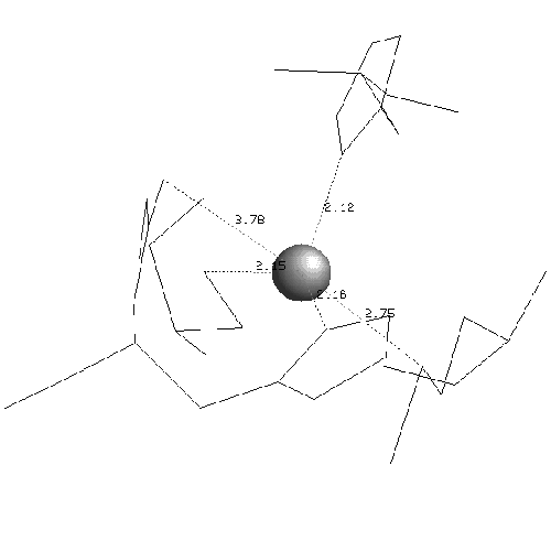
|
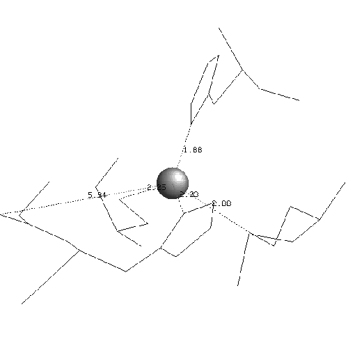
|
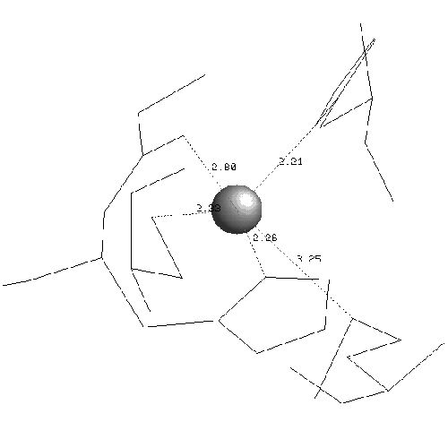
|
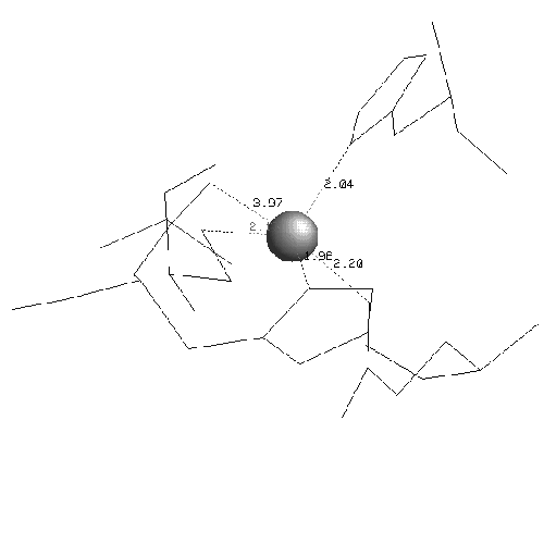
|
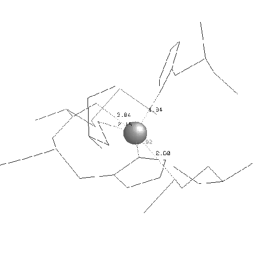
|
2002-04-09